
A post by Emma Tarmey, PhD student on the Compass programme.
This blog post serves as an introduction to the problem of confounder handling within the broader topic of covariate selection and model selection for causal inference purposes. In this post, we begin with a motivating example, describe the problem of confounding, describe current solutions to the problem and how statistical solution methods compare to knowledge-based solution methods. It is intended that readers come away from this article understanding which use cases each of the solution methods are intended for, as well as what advantages and disadvantages each method provides.
Introduction
There exists a common saying, “correlation does not imply causation”. This phrase is often used when discussing statistical analyses to describe the idea that just because two phenomena or patterns often appear together, does not automatically mean that one necessarily causes the other. There are a number of reasons why two events, A and B, may occur together, with “A causes B” being only one of several explanations for the observed correlation. In epidemiology, substantiating a causal claim, “causal inference”, can be highly valuable towards determining medical best practice and testing the effectiveness of medical treatments and interventions. A correlation between two events, A and B, may be distorted or even fabricated whole-cloth by the influence of an outside event C, which mutually causes both. As such, particularly in the context of clinical trials for medical treatments, verifying that no such outside influences are distorting our results is essential for producing valid causal inferences.
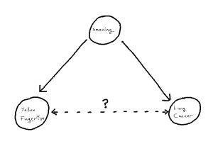
Yellow Fingers and Lung Cancer
To motivate the idea of a distorted correlation from the introduction, we look to a famous example: the association between the yellowing at the tip’s of ones fingers and incidence of lung cancer.[1][2] We observe from the literature that, when attempting to predict incidence of lung cancer, the yellowing of ones finger tips makes an excellent predictor variable.[1] However, there is no causal link between these two events, instead, both the yellowing and lung cancer are mutually caused by smoking.[2] This, in turn, creates an unhelpful statistical association between the two variables, one which is then correctly estimated in modelling but no longer corresponds just to our causal pathway. As such, when attempting to understand causal factors to lung cancer, it becomes important not to declare yellowing as a cause despite the fact that yellowing may “look like a cause” based on the data itself.
One can imagine, in an isolated example like this, it can be straight-forward to detect this from first principles using the existing causal knowledge we have. But, if for example a given study has not recorded smoking as a variable, we become unable to identify the phenomenon and thus unable to correctly attribute the source of our statistical associations. The phenomenon within causal structures of a common cause is referred to as “confounding”, thus giving us the sub-problem of “confounder handling” when attempting to use our statistical models for causal inference. Notably, causal pathways can be more complex than the above example. If we have a longer pathway by which we add to the statistical association between X and Y, any such covariate on that pathway is a potential confounder, whose adjustment will solve our problem. We define our problem formally as follows:
Problem: Confounder Handling
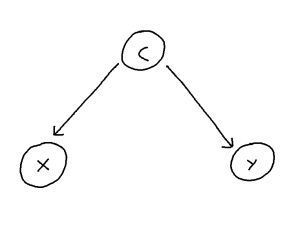
Confounding is defined as the phenomenon within any causal structure wherein both an exposure (input variable) and outcome (output variable) are mutually caused by a third outside variable (the confounder). This in turn creates a statistical association between the two covariates which is not attributable to a causal pathway from X to Y. This phenomenon takes the following general shape:
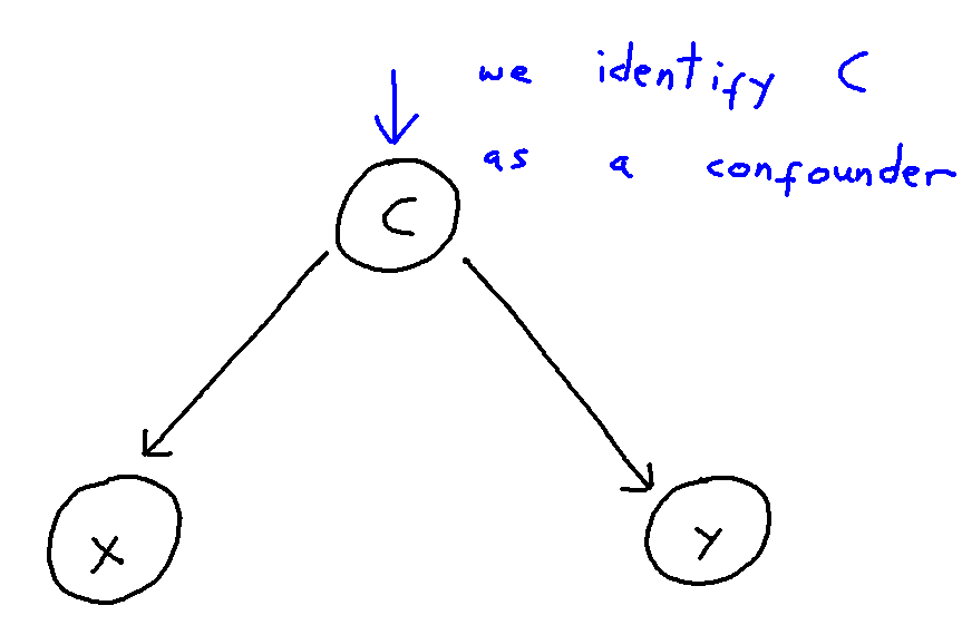
It can be helpful to think of confounder-handling as containing two sub-problems which we solve together:
- Confounder Identification: Identifying the set of all covariates which act as confounders within a given causal structure
- Control-Set Selection: Selecting an optimal (by some criterion) subset of these identified confounders to include in the model to best control for confounding
This problem can be though of in the following way:
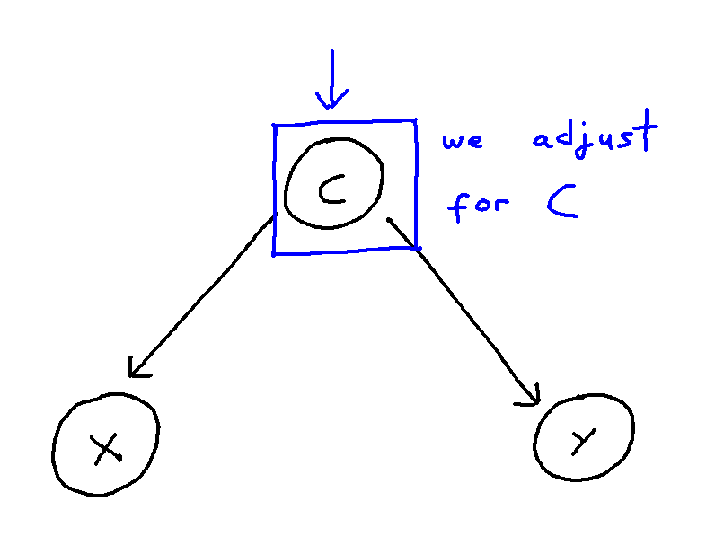
We may control for a variable by means of including it within our regression or remove the influence of a variable altogether by stratifying our data. These, in turn, both remove the statistical association attributable to confounding. However, when the causal structure is larger and more complex, correctly handling confounding becomes trickier. Firstly, we risk inducing “selection”, and thus creating more confounding pathways, if we adjust for covariate which confounds the X-Y relationship but is itself also caused by other covariates. Secondly, if we adjust for an “instrument” of X, that being a covariate Z which is a cause of X but not of Y, then we risk amplifying bias from unseen confounding. Thirdly, further issues arise if many covariates within the model are correlated with each other, as then estimating a given causal effect becomes much more difficult, even for an unconfounded model.
Additionally, though this may seem to go without saying, we only have the variables that we have. Unmeasured confounding, from a covariate not within our dataset, can very much produce the same distortions but also be impossible to control for. With all this in mind, we look to the existing solutions to these above problems.
Solution: Confounder-Handling
There exist two broad solution types to the problem of confounder-handling, those being:
- A direct approach working from causal knowledge
- An indirect approach working from observed data
Existing knowledge-based solutions include:
- Back-door path criterion: [3]
- The back-door path criterion states that the causal effect is identifiable if there does not exist any “back door path” connecting the exposure X and outcome Y within the causal structure.
- As such, we may prevent confounding by controlling a variable present on any such existing path to “block” this path and thus prevent confounding via that path.
- Front-door path criterion: [3]
- The front-door path criterion states that the causal effect is identifiable (our statistical association is still a consistent estimator of the causal effect), even if the backdoor path criterion isn’t strictly satisfied. If we have a “mediator” covariate M, a covariate which sits between two covariates creating a direct path via itself, between X and Y, the the X-Y causal effect remains identifiable if we satisfy all of the following:
- M intercepts all causal pathways from X to Y
- There does not exist any backdoor path between X and M
- X blocks every backdoor path from M to Y
- The front-door path criterion states that the causal effect is identifiable (our statistical association is still a consistent estimator of the causal effect), even if the backdoor path criterion isn’t strictly satisfied. If we have a “mediator” covariate M, a covariate which sits between two covariates creating a direct path via itself, between X and Y, the the X-Y causal effect remains identifiable if we satisfy all of the following:
- Pre-treatment criterion: [4]
- The pre-treatment criterion states that, if we control for all covariates which occur prior to the exposure X in time, then we must necessarily have controlled for all confounders, and thus our causal effect is identifiable.
- Common-cause criterion : [4]
- The common-cause criterion states that, if we control for any and all covariates who mutually cause both the exposure X and outcome Y, then we must necessarily have controlled for all confounders.
- (Twice-modified) Disjunctive-cause criterion: [4]
- The (twice-modified) disjunctive cause criterion states that we can construct a sufficient adjustment set S in the following way:
- Add to our set S any pre-exposure covariate which is a cause of X, Y or both
- Remove from S any covariate Z which acts as an instrument of X
- Add to S any covariate which, though not satisfying condition 1, can act as a good proxy for unmeasured confounders of the X-Y relationship
- The (twice-modified) disjunctive cause criterion states that we can construct a sufficient adjustment set S in the following way:
- District criterion (iterative graph expansion): [5]
- The district criterion states that we have controlled for confounding if we our adjustment set S does indeed leave covariates X and Y in separate “districts” of a specially defined sub-graph of our wider causal structure, the setup of which is beyond the scope of this blog article.
- This criterion forms the theoretical justification to the method of iterative graph expansion proposed in the same paper, which readers are encouraged to find from the references if they would like to learn more.
Existing statistically-based solutions include:
- Step-wise regression: [6]
- Stepwise regression is a variable selection and model fitting procedure, which works by means of iteratively adding and removing explanatory variables (covariates other than X and Y) to form an optimal model where all explanatory variables are considered significant by some outside significance criterion (such as AIC).
- LASSO (Least absolute shrinkage and selection operator): [7]
- LASSO is a parameter estimation procedure typically employed for variable selection, which can be employed similarly for confounder identification.
More bespoke statistical solutions include:
- Change-in-estimate approach: [8]
- The change in estimate approach detects confounding via statistical significance testing, iteratively as covariates are added and removed. The idea, intuitively, is that if removing an outside variable as explanatory has a significant impact on the X-Y relationship, then it was likely confounding the two, and is identified as such.
- Targeted maximum likelihood estimators: [9]
- Targeted maximum likelihood estimators (TMLEs) are doubly-robust parameter estimators, which can be used for determining regression coefficients for statistical models while optimizing the bias-variance trade-off. This is used for confounder identification similarly to LASSO.
We have seen many approaches to the problem, but which is best? In thinking this through, we conclude that which approach is best depends on one’s intended use case. Specifically:
- Whether or not causal knowledge is available, with causal methods preferred as these provide guarantees of unconfoundedness in the result
- If causal knowledge is available, how much? Are we able to fully enumerate our problem?
Since different knowledge-based methods require different amounts of causal knowledge and provide stronger and weaker results correspondingly, it makes sense to select the approach most suited to the DAG we’re presently examining. However, knowledge-based methods scale poorly to larger causal structures, both in terms of running their algorithms and of enumerating the DAG to begin with – they quickly become intractable. Hence – statistical approaches, which provide weaker results with regards to unconfoundedness, but scale much better to larger causal scenarios and in principle require no causal knowledge to execute.
Conclusion
In conclusion, there exists a problem of confounding within the field of causal inference, and different solutions to this problem offer different advantages and disadvantages. Which solution is necessarily “best” depends upon your use case, specifically size of use-case and amount of causal knowledge available.
Contact Details
Miss Emma Jane Tarmey (she/her), University of Bristol, emma.tarmey@bristol.ac.uk
References
- Smith, George Davey and Phillips, Andrew N. Confounding in epidemiological studies: why ”independent” effects may not be all they seem. British Medical Journal, 305(6856):757–759, September 1992.
- Rothman, Kenneth J. et al. Serum Beta-Carotene: A Mechanism or ”Yellow Finger”? Epidemiology, 3(4):277–279, July 1992.
- Pearl, Judea. Causal diagrams for empirical research. Biometrika, 82(4):669–710, 1995.
- VanderWeele, Tyler J. Principles of Confounder Selection. European Journal of Epidemiology, 34:211–219, 2019, Section 4
- F. Richard Guo and Qingyuan Zhao. Confounder Selection via Iterative Graph Expansion. arXiv, October 2023
- VanderWeele, Tyler J. Principles of Confounder Selection. European Journal of Epidemiology, 34:211–219, 2019, Section 5
- Susan M. Shortreed and Ashkan Ertefaie. Outcome-Adaptive Lasso: Variable Selection for Causal Inference. Biometrics, 73:1111–1122, 2017. Publisher: Wiley.
- Talbot, Denis and Diop, Awa and Lavigne-Robichaud, Mathilde and Brisson, Chantal. The change in estimate method for selecting confounders: A simulation study. Statistical Methods in Medical Research 30(9):2032–2044, 2021.
- Schuler, Megan S. and Rose, Sherri. Targeted Maximum Likelihood Estimation for Causal Inference in Observational Studies. American Journal of Epidemiology, 185(1):65–73, January 2017.
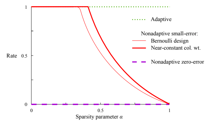 A graph comparing different group testing designs, where the $\text{Rate} = \log_2\binom{n}{k}/T$ where $T$ is the number of tests needed to recover all the defective items (with high probability for the red lines and with certainty for the purple line). [1]


 with a particular sequence, we can take a sample from this synthesis and analyse it via mass spectrometry. In this process, molecules in the sample are first fragmented — broken apart into ions — and these charged fragments are then passed through an electromagnetic field. The trajectory of each fragment through this field depends on its mass/charge ratio (m/z), so measuring these trajectories (e.g. by measuring time of flight before hitting some detector) allows us to calculate the m/z of fragments in the sample. This gives us a discrete mass spectrum: counts of detected fragments (intensity) across a range of m/z bins [5].
 every product of a single fragmentation of
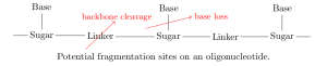
 , where
  is the intensity in the
  bin. For a set
  of possible fragments, let
  be the amount of
  that is actually present. We would like to estimate the amounts of each fragment based on the spectrum
  .
. and
and  and this produced a spectrum
  , we can say the intensity contributed to bin
  by
by  In mass spectrometry, the intensity in a single bin due to a single fragment is linear in the amount of that fragment, and the intensities in a single bin due to different fragments are additive, so in some general spectrum we have
 such that
  (so the columns of
  correspond to fragments in
  solves
  . In practice this exact solution is not found — due to experimental noise and potentially because there are contaminant fragments in the sample not included in
  for which
  is close to
  -normalise these columns, meaning the total intensity (over all bins) of each fragment in the library matrix is uniform, and so the values in
  can be directly interpreted as relative abundances of each fragment.
 which maximises the likelihood of the system is approximated by the iterative formula
}=\left(\mathbf A^T \frac{\mathbf b}{\mathbf{A\hat x}^{(t)}}\right)\odot \mathbf{\hat x}^{(t)}.")
 represent (respectively) elementwise division and multiplication of two vectors. This is known as the Richardson-Lucy algorithm [9].
}=\left(\mathbf A^T \frac{\mathbf b}{\mathbf{A\hat x}^{(t)}}\right)\odot \frac{ \mathbf{\hat x}^{(t)}}{\mathbf 1 + \lambda},")
 is a regularisation parameter [10].
 , we smooth and bin the m/z values of the most abundant isotopes of
  , and store these values in the columns of
  ) for clarity.