
A post by Conor Crilly, PhD student on the Compass programme.
Introduction
This project investigates uncertainty quantification methods for expensive computer experiments. It is supervised by Oliver Johnson of the University of Bristol, and is partially funded by AWE.
Outline
Physical systems and experiments are commonly represented, albeit approximately, using mathematical models implemented via computer code. This code, referred to as a simulator, often cannot be expressed in closed form, and is treated as a ‘black-box’. Such simulators arise in a range of application domains, for example engineering, climate science and medicine. Ultimately, we are interested in using simulators to aid some decision making process. However, for decisions made using the simulator to be credible, it is necessary to understand and quantify different sources of uncertainty induced by using the simulator. Running the simulator for a range of input combinations is what we call a computer experiment [1]. As the simulators of interest are expensive, the available data is usually scarce. Emulation is the process of using a statistical model (an emulator) to approximate our computer code and provide an estimate of the associated uncertainty.
Intuitively, an emulator must possess two fundamental properties
- It must be cheap, relative to the code
- It must provide an estimate of the uncertainty in its output
A common choice of emulator is the Gaussian process emulator, which is discussed extensively in [2] and described in the next section.
Types of Uncertainty
There are many types of uncertainty associated with the use of simulators including input, model and observational uncertainty. One type of uncertainty induced by using an expensive simulator is code uncertainty, described by Kennedy and O’Hagan in their seminal paper on calibration [3]. To paraphrase Kennedy and O’Hagan: In principle the simulator encodes a relationship between a set of inputs and a set of outputs, which we could evaluate for any given combination of inputs. However, in practice, it is not feasible to run the simulator for every combination, so acknowledging the uncertainty in the code output is required.
Gaussian Processes
Suppose we are interested only in investigating code uncertainty, that is, we simply want to predict the code output for some untried combinations of control inputs. We denote our simulator by ")


Treating our code 
Definition 1: A Gaussian process is a collection of random variables, any finite combination of which have a multivariate Gaussian distribution.
Analogously to a multivariate Gaussian, which is fully specified by its mean 

")
")
A 
 \sim \mathcal{GP}(m(x), k(x,x')).")
Prior
To clarify how Definition 1 relates to emulation of our simulator, the random variables in Definition 1 correspond to the values of the function
- Choose your favourite index points
- Choose your mean function
and kernel function
, specifying any hyperparameters
- Calculate the covariance matrix
- By definition,
- Simulate an
dimensional vector
, where
- Plot each of the points

")

")
")
Posterior
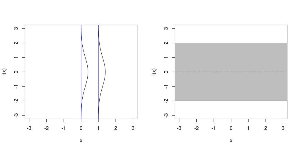
Suppose we are interested in emulating some function. For illustration we can simulate some `toy’ data from the function  = \frac{3}{2}(\sin(\frac{x}{3}) + \cos(\frac{x}{3}))")


\Sigma(x_{tr}, x_{tr})^{-1}f_{tr}")
 - \Sigma(x_{te}, x_{tr})\Sigma(x_{tr}, x_{tr})^{-1}\Sigma(x_{tr}, x_{te})")
With minor adjustments the same process as we used for the prior can be used to draw `functions’ from the posterior, ")
This simple conditioning procedure also works if we assume that observations are made with some additive Gaussian noise. However, when our likelihood is non-Gaussian, for example when using Gaussian processes for classification, difficulties arise. In particular, our posterior is no longer Gaussian and its derivation involves intractable integrals;

Constrained GPs
Standard
Notice that both monotonicity and convexity of a function can be specified in terms of derivatives thereof. One useful theorem is that 


")
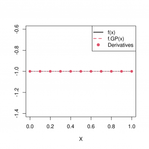
This approach is only useful if we actually observe the derivatives (equality constraints), and we illustrate in Figure 3 how this can improve emulation of the function  = -\frac{1}{8}\big((2x -1)^2 -1\big)")
Several approaches have been proposed in the literature to tackle the case where we do not observe the derivatives, which would be the case if we could only assume monotonicity [7]. In [7], indicator variables are used at predefined inputs to indicate whether or not the derivative is positive. Inference is then made conditional on these indicator variables. One issue with this approach is that sample paths are not guaranteed to obey the desired constraints at all points in the domain 

Conclusion
This was a brief introduction to
References
[1] J. Sacks, W. J. Welch, T. J. Mitchell, and H. P. Wynn. Design and analysis of computer experiments. Statistical Science, 4(4):409–423, Nov 1989.
[2] C. E. Rasmussen and C. K. I. Williams. Gaussian Processes For Machine Learning. The MIT Press, Cambridge 2006.
[3] M. C. Kennedy and A. O’Hagan. Bayesian calibration of computer models. Journal of the Royal Statistical Society: Series B (Statistical Methodology), 63(3):425–464, 2001.
[4] T. J. Santner, B. J. Williams, and W. I. Notz. The Design and Analysis of Computer Experiments. Springer Series in Statistics. Springer, 2003.
[5] ST John. Gaussian processes for non-gaussian likelihoods. Gaussian Process Summer School 2021. http://gpss.cc/gpss21/slides/John2021.pdf.
[6] C. Jidling, N. Wahlström, A. Wills, and T. B. Schön. Linearly constrained gaussian processes. In Advances in Neural Information Processing Systems, volume 30. Curran Associates, Inc., 2017.
[7] S. Golchi, D. R. Bingham, H. Chipman, and D. A. Campbell. Monotone emulation of computer experiments. SIAM/ASA Journal on Uncertainty Quantification, 3(1):370–392, Jan 2015.
[8] L. Swiler, M. Gulian, A. Frankel, C. Safta, and J. Jakeman. A survey of constrained gaussian process regression: Approaches and implementation challenges. Journal of Machine Learning for Modeling and Computing, 1(2):119–156, 2020. ISSN 2689-3967. doi: 10.1615/JMachLearnModelComput.2020035155.