Student Perspectives: Embedding probability distributions in RKHSs

A post by Jake Spiteri, Compass PhD student.

Recent advancements in kernel methods have introduced a framework for nonparametric statistics by embedding and manipulating probability distributions in Hilbert spaces. In this blog post we will look at how to embed marginal and conditional distributions, and how to perform probability operations such as the sum, product, and Bayes’ rule with embeddings.

Embedding marginal distributions

Throughout this blog post we will make use of reproducing kernel Hilbert spaces (RKHS). A reproducing kernel Hilbert space is simply a Hilbert space with some additional structure, and a Hilbert space is just a topological vector space equipped with an inner product, which is also complete.

We will frequently refer to a random variable $X$ which has domain $\mathcal{X}$ endowed with the $\sigma$ -algebra $\mathcal{B}_\mathcal{X}$ .

Definition. A reproducing kernel Hilbert space $\mathcal{H}$ on $\mathcal{X}$ with associated positive semi-definite kernel function $k: \mathcal{X} \times \mathcal{X} \rightarrow \mathbb{R}$ is a Hilbert space of functions $f: \mathcal{X} \rightarrow \mathbb{R}$ . The inner product $\langle\cdot,\cdot\rangle_\mathcal{H}$ satisfies the reproducing property: $\langle f, k(x, \cdot) \rangle_\mathcal{H}, \forall f \in \mathcal{H}, x \in \mathcal{X}$ . We also have $k(x, \cdot) \in \mathcal{H}, \forall x \in \mathcal{X}$ .

It may be helpful to think of $\mathcal{H}$ as $\overline{\text{span}\{k(x, \cdot)\}}$ ; all functions in our space may be written as a sum of feature maps $k(x, \cdot)$ . This can help us visualise what functions belong to our RKHS. We should also note that kernel functions are not limited to $\mathcal{X} = \mathbb{R}^d$ — kernel functions have been defined for inputs such as strings, graphs, images, etc.

Definition. Let $\mathcal{P}(\mathcal{X})$ the space of all probability measures on $\mathcal{X}$ . We can embed any probability distribution $\mathbb{P} \in \mathcal{P}(\mathcal{X})$ into the RKHS $\mathcal{H}$ with associated kernel $k$ via the kernel mean embedding:

$\mu_\mathbb{P}: \mathcal{P}(\mathcal{X}) \rightarrow \mathcal{H}, \quad \mu_\mathbb{P}: \mathbb{P} \mapsto \int k(x, \cdot) d\mathbb{P}(x)$

The embedding $\mu_\mathbb{P}$ exists and belongs to the RKHS $\mathcal{H}$ if $\mathbb{E}_\mathbb{P}[\sqrt{k(X,X)}] < \infty$ . The kernel mean embedding is representer of expectation in the RKHS: it satisfies the reproducing property $\mathbb{E}_\mathbb{P}[f(X)] = \langle f, \mu_\mathbb{P} \rangle_\mathcal{H}, \forall f \in \mathcal{H}$ . I.e. can compute expectations of functions $f \in \mathcal{H}$ with respect to $\mathbb{P}$ by taking an inner product between $f$ and $\mu_\mathbb{P}$ .

A useful property of the kernel mean embedding is that it captures all characteristics of a probability distribution, for a good choice of kernel. Provided that the feature mapping induced by the kernel is injective, the embedding is unique. A kernel which corresponds to an injective feature mapping is said to be characteristic. That is, for $\mathbb{P}, \mathbb{Q} \in \mathcal{P}(\mathcal{X})$ , if $\mu_\mathbb{P} = \mu_\mathbb{Q}$ then we must have $\mathbb{P} = \mathbb{Q}$ for a characteristic kernel. Choosing an appropriate kernel function for a given problem is not straightfoward, and it is common to use a ‘default’ kernel choice such as the Gaussian or Laplace kernel, as they are characteristic. We should note here that whilst the mapping from distribution to kernel mean embedding is unique, reconstructing the original density function is non-trivial.

Empirical estimator. In practice it is unlikely that we would have access to the distribution $\mathbb{P}$ , and so rather than compute the kernel mean embedding $\mu_\mathbb{P}$ , we can only compute its empirical estimate. Given an i.i.d. sample $\{x_1, \dots, x_n\}$ from $\mathbb{P}$ , we can compute the unbiased estimate $\hat{\mu}_\mathbb{P} := \frac{1}{n} \sum_{i=1}^n k(x_i, \cdot)$ . This empirical estimator has $\sqrt{n}$ -consistency.

Above we have introduced a quantity which makes use of the mean feature mapping in the RKHS. Similarly, we may also make use of the covariance of feature mappings in the RKHS.

Definition. Let $(X, Y)$ be a random variable taking values on domain $\mathcal{X} \times \mathcal{Y}$ , and let $\mathcal{H}$ and $\mathcal{G}$ be RKHSs with kernel functions $k$ and $l$ on domains $\mathcal{X}$ and $\mathcal{Y}$ respectively. Let $\phi(x) := k(x, \cdot)$ and $\varphi(y) := l(y, \cdot)$ be the feature maps corresponding to kernels $k$ and $l$ respectively. Then we define the (uncentered) cross-covariance operator $\mathcal{C}_{YX}: \mathcal{H} \rightarrow \mathcal{G}$ as

$\mathcal{C}_{YX} := \mathbb{E}_{\mathbb{P}_{YX}}[\varphi(Y) \otimes \phi(X)],$

where $\otimes$ denotes the tensor product, and $\mathbb{P}_{YX}$ denotes the joint probability distribution of $(X, Y).$

The cross-covariance operator exists if $\mathbb{E}_X[k(X, X)] < \infty$ and $\mathbb{E}_Y[l(Y, Y)] < \infty$ . It is useful to note that $\mathcal{C}_{YX}$ can be identified as the kernel mean embedding of the joint distribution in the tensor product space $\mathcal{G} \otimes \mathcal{H}$ . We emphasise that the cross-covariance operator is an operator mapping from one RKHS to another. We see that when acting on an element $f \in \mathcal{H}$ we have $\mathcal{C}_{YX}(f)= \mathbb{E}_{\mathbb{P}_{YX}}[\varphi(Y) \langle f, \phi(X) \rangle_\mathcal{H}]\in\mathcal{G}$ .

Empirical estimator. Given an i.i.d. sample $\{x_i, y_i\}_{i=1}^n$ from the joint probability distribution $\mathbb{P}_{XY},$ we have the following empirical estimator of the cross-covariance

$\hat{\mathcal{C}}_{YX} = \frac{1}{n} \Phi^T \Upsilon,$

where $\Phi = [ \phi(x_1), \dots, \phi(x_n)] \in \mathcal{H}^n$ and $\Upsilon = [ \varphi(y_1), \dots, \varphi(y_n)] \in \mathcal{G}^n$ are row vectors of functions in $\mathcal{H}$ and $\mathcal{G}$ respectively.

Embedding conditional distributions

Using the cross-covariance operator, we can now define the conditional mean embedding. We want to extend the notion of embedding a marginal distribution $P(X)$ to that of embedding a conditional distribution $P(Y | X)$ and $P(Y | X = x)$ for some $x \in \mathcal{X}$ . Embeddings which capture the dependence between variables will allow us to develop more complex algorithms, and will allow us to produce kernel versions of elementary probability operations such as the sum rule and product rule.

We start by specifying two conditions which we want the conditional mean embedding to satisfy based on our definiton of the kernel mean embedding. We will use $\mu_{Y | X=x} \in \mathcal{G}$ and $\mathcal{U}_{Y|X}:\mathcal{H} \rightarrow \mathcal{G}$ to denote the embeddings of the conditional distributions $P(Y | X = x)$ and $P(Y | X)$ respectively.

These conditions are

$\mu_{Y | X=x} = \mathbb{E}_{Y | X=x}[\varphi(Y) | X = x] = \mathcal{U}_{Y|X} k(x, \cdot), \quad \forall x\in\mathcal{X}$ .
$\mathbb{E}_{Y | X=x}[g(Y) | X = x] = \langle g, \mu_{Y|X=x} \rangle_\mathcal{G}, \quad \forall g \in \mathcal{G}$

Note that for a given $x \in \mathcal{X}$ the embedding of $P(Y | X = x)$ , $\mu_{Y | X=x}$ , is an element in $\mathcal{G}$ , whereas the embedding of $P(Y | X)$ , $\mathcal{U}_{Y|X}$ , is an operator which traces out a family of elements in the RKHS $\mathcal{G}$ .

It is shown in (Song, 2009) that the following definition satisfies the above properties.

Definition. Let $\mathcal{C}_{XX}: \mathcal{H} \rightarrow \mathcal{H}$ , and $\mathcal{C}_{YX}: \mathcal{H} \rightarrow \mathcal{G}$ . Then we can define the conditional mean embeddings of the conditional distributions $P(Y | X)$ and $P(Y | X = x)$ , for $x \in \mathcal{X}$ , as

$\mathcal{U}_{Y|X} := \mathcal{C}_{YX} \mathcal{C}_{XX}^{-1}, \quad \mu_{Y | X=x} := \mathcal{C}_{YX} \mathcal{C}_{XX}^{-1} k(x, \cdot),$

under the assumption that $\mathbb{E}_{Y|X}[g(Y) | X] \in \mathcal{H}$ . It is easy to produce examples in which this does not hold, and so we often replace the above inverse with a Tikhonov-regularised inverse, and consider the embeddings to be approximations of the true embeddings.

Empirical estimator. Given a set of i.i.d. samples $\{x_i, y_i\}_{i=1}^n$ from the joint distribution $P(X,Y)$ , the conditional mean embedding can be estimated using

$\hat{\mu}_{Y|X=x} = \sum_{i=1}^n \beta_i l(y_i, \cdot)$ ,

where $\beta := (K + n \lambda I)^{-1} k_x \in \mathbb{R}^n$ for $K\in\mathbb{R}^{n \times n}$ the Gram matrix associated with $\{ x_1, \dots, x_n\}$ , and $k_x = [k(x, x_1), \dots, k(x, x_n)]$ , and $\lambda$ a regularisation parameter.

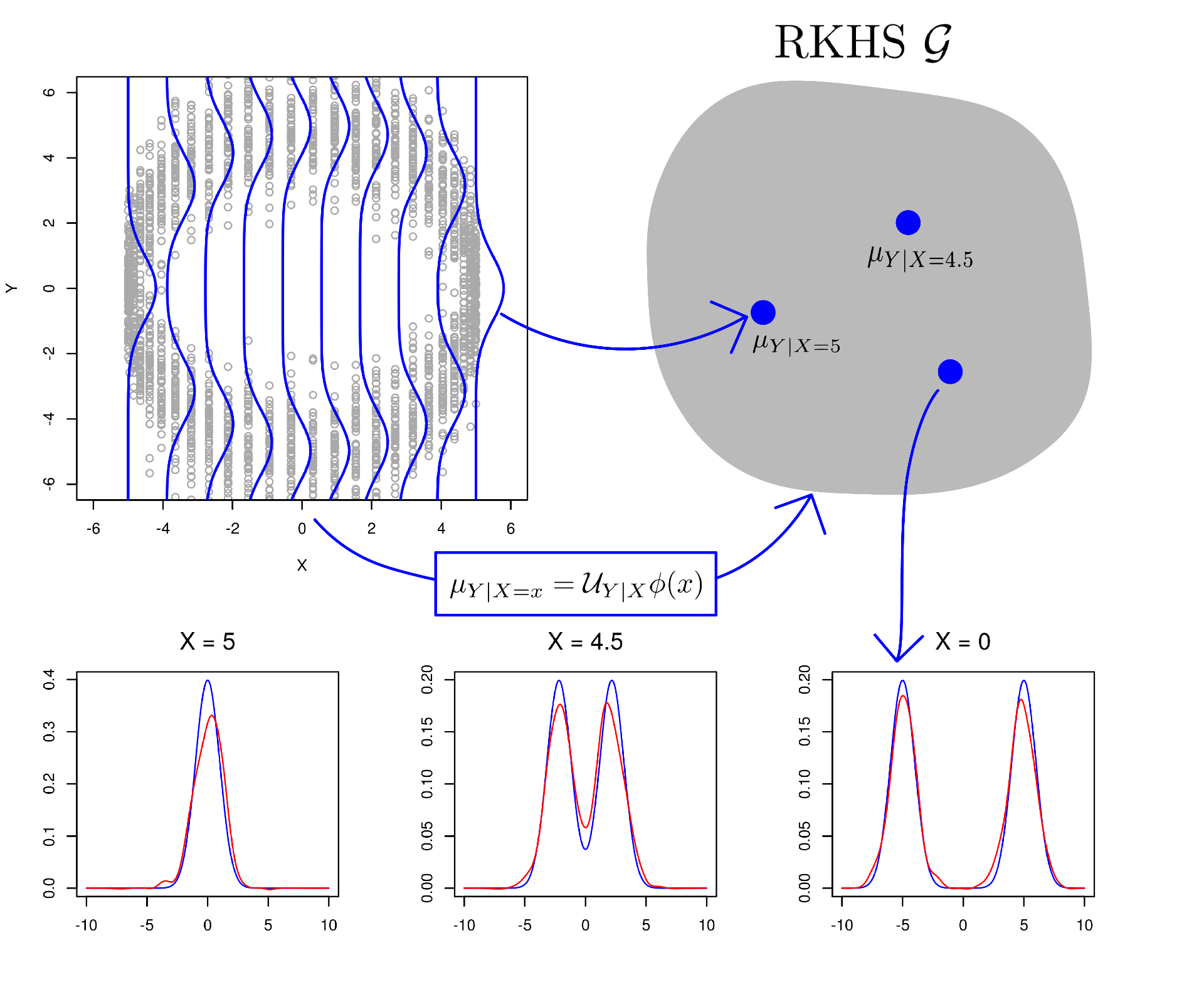
An example. Here we look at a simple example of the conditional mean embedding. We generate data in a method inspired by Schuster et al. (2020). We start by drawing a circle on the $(x,y)$ -plane, and specifying 50 equidistant points on the circle. Each of these points is the mean of a Gaussian distribution over $Y$ , and we draw 50 samples from each distribution with equal probability. The conditional distribution $P(Y | X)$ in this scenario is a mixture of Gaussians. The top left plot of Figure 1 shows the data sampled from these Gaussians in grey, with conditional distributions overlaid in blue. The conditional mean embedding embeds each conditional distribution in the RKHS $\mathcal{G}$ illustrated in the top right plot, via $\mu_{Y|X=x} = \mathcal{U}_{Y|X} \phi(x)$ . In the second row of Figure 1 we see three examples of the reconstructed conditional densities in red. These reconstructed densities have been obtained via the nonparametric estimator proposed in Kanagawa et al. (2014).

Figure 1. A visualisation of the conditional mean embedding.

Operations: the Sum, Product, and Bayes’ rule

Using the conditional mean embedding and the cross-covariance operator, we can produce versions of the sum, product, and Bayes’ rule which allow us to manipulate distributions embedded in an RKHS.

Recall the sum rule and product rule: $P(X) = \sum_{Y \in \mathcal{Y}} P(X, Y)$ , and $P(X, Y) = P(Y | X) P(X)$ .

Kernel Sum rule. The sum rule allows us to compute the marginal density of a variable $X$ given the joint distribution over variables $X$ and $Y$ , by marginalising out $Y$ .

Using the law of total expectation, we have $\mu_X = \mathbb{E}_{XY}[\varphi(X)] = \mathbb{E}_Y \mathbb{E}_{X | Y}[\varphi(X)|Y]$ . Thus, we have

$\mu_X = \mathcal{U}_{X|Y} \mathbb{E}_Y [\phi(Y)] = \mathcal{U}_{X|Y} \mu_Y$ .

Kernel Product rule. To construct a kernel product rule, we consider the tensor product feature map $\varphi(X) \otimes \phi(Y)$ . We can factorise the embedding $\mu_{XY} = \mathbb{E}_{XY}[\varphi(X) \otimes \phi(Y)]$ in two ways using the law of total expectation

$\mathbb{E}_Y \mathbb{E}_{X | Y} [\varphi(X) \otimes \phi(Y) | Y] = \mathcal{U}_{X | Y} \mathbb{E}_Y[\phi(Y) \otimes \phi(Y)]$ ,
$\mathbb{E}_X \mathbb{E}_{Y | X} [\phi(Y) \otimes \varphi(X)| X] = \mathcal{U}_{Y | X} \mathbb{E}_X[\varphi(X) \otimes \varphi(X)]$ .

Let $\mu_Y^\otimes := \mathbb{E}_Y[\phi(Y) \otimes \phi(Y)]$ , and $\mu_X^\otimes := \mathbb{E}_X[\varphi(X) \otimes \varphi(X)]$ . Then we can rewrite the above as

$\mu_{XY} = \mathcal{U}_{X | Y} \mu_Y^\otimes = \mathcal{U}_{Y | X}\mu_X^\otimes$ .

This looks similar to the sum rule, but we see that there is an additional copy of the variables $Y$ and $X$ passed as input, which is not marginalised out as is done in the sum rule.

Kernel Bayes rule. The kernel Bayes’ rule (KBR) is a nonparametric method which allows for Bayesian inference in the absence of a parametric model or likelihood. In KBR we embed the prior and likelihood in an RKHS via the kernel mean embedding and cross-covariance operator respectively, and use the sum and product rules to manipulate the embeddings in the RKHS.

The presentation of KBR shown here is that given in Muandet et al. (2017), which provides a concise summary of the original work (Fukumizu et al., 2013). Our aim is to compute the embedding of the posterior $P(Y|X)$ given a prior distribution $\Pi(Y)$ . We obtain the embedding of the posterior distribution as $\mu_{Y | X=x} = \mathcal{U}_{Y | X}^\Pi \varphi(x)$ , where we use a superscript $\Pi$ to denote dependence on the prior $\Pi(Y)$ . More precisely, we have

$\mu_{Y | X=x} = \mathcal{U}_{Y | X}^\Pi \varphi(x) = \mathcal{C}_{YX}^\Pi (\mathcal{C}_{XX}^\Pi)^{-1} \varphi(x)$ ,

where the cross-covariance operators depend on the prior, and are given by

$\mathcal{C}_{YX}^\Pi = (\mathcal{U}_{X | Y} \mathcal{C}_{YY}^\Pi)^{T}, \quad \mathcal{C}_{XX}^\Pi = \mathcal{U}_{(XX) | Y} \mu_Y^\Pi$ .

These results follow from the product and sum rule respectively, where we have replaced the input feature map $\varphi(X)$ with the tensor product feature map $\varphi(X) \otimes \varphi(X)$ . The embeddings $\mu_Y^\Pi$ and $\mathcal{C}_{YY}^\Pi$ are simply the embedded prior distribution corresponding to the feature maps $\phi(Y)$ and $\phi(Y) \otimes \phi(Y)$ .

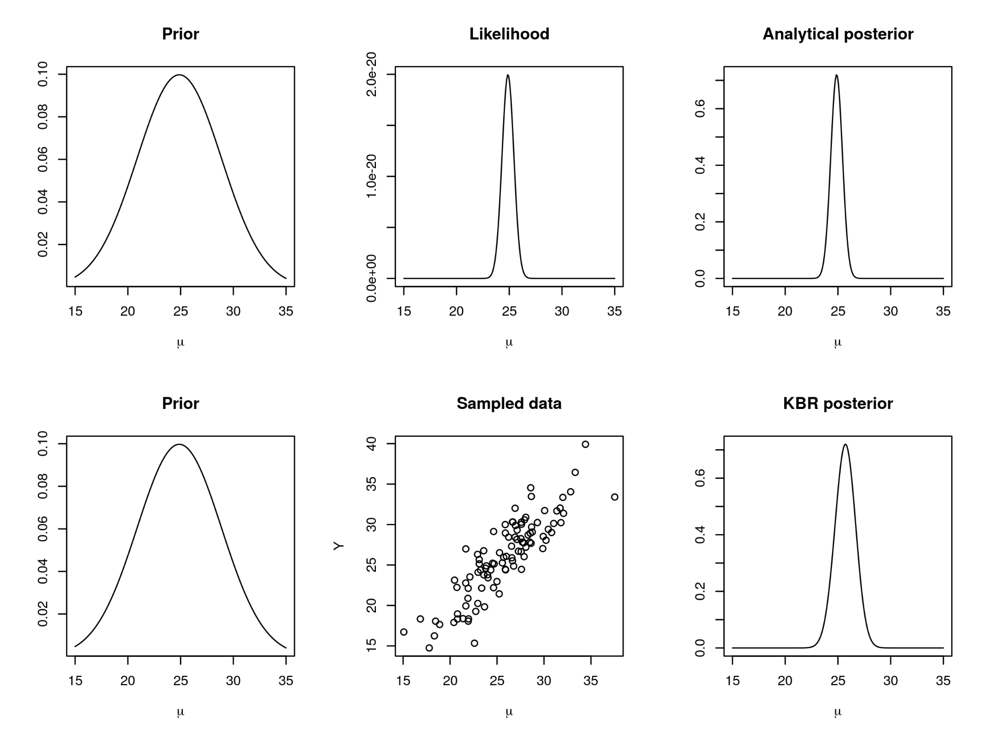
A KBR example. Here we look at a simple example of Bayesian inference without a likelihood, similar to that given in Fukumizu et al. (2013). In this toy example we assume that we cannot write down the likelihood function, but we can sample from it. We generate data from a Normal distribution with mean $\mu = 25$ , and we assume the variance $\sigma^2 = 2.5^2$ is known. We place a Normal prior on $\mu$ with mean equal to the mean of the observed data, and standard deviation 4. Figure 2 below shows two ways of approaching posterior inference: in the first row we use the fact that the prior and likelihood are conjugate, and we derive the analytical posterior distribution; in the second row we embed the prior distribution and the joint distribution in the RKHS and use KBR to obtain an embedding of the posterior.

Figure 2. Top row: Posterior inference when the prior and likelihood are conjugate. Bottom row: Posterior inference via KBR when the likelihood is intractable.

References

Fukumizu, K., L. Song, and A. Gretton (2013). “Kernel Bayes’ rule: Bayesian inference with positive definite kernels”. In: The Journal of Machine Learning Research 14.1, pp. 3753–3783.
Kanagawa, M. and K. Fukumizu (2014). “Recovering distributions from Gaussian RKHS embeddings”. In: Artificial Intelligence and Statistics. PMLR, pp. 457–465.
Muandet, K., K. Fukumizu, B. Sriperumbudur, and B. Schölkopf (2017). “Kernel Mean Embedding of Distributions: A Review and Beyond”. In: Foundations and Trends in Machine Learning.
Schuster, I., M. Mollenhauer, S. Klus, and K. Muandet (2020). “Kernel conditional density operators”. In: International Conference on Artificial Intelligence and Statistics. PMLR, pp. 993–1004.
Song, L., J. Huang, A. Smola, and K. Fukumizu (2009). “Hilbert space embeddings of conditional distributions with applications to dynamical systems”. In: Proceedings of the 26th Annual International Conference on Machine
Learning, pp. 961–968.