Sensitivity analysis seeks to understand how much changes in each input affect the output of a model. We want to be able to determine how variation in a model’s output can be attributed to variations in its input. Given the high amount of uncertainty present in most real-world modelling settings, it is crucial to understand the magnitude of this uncertainty’s impact on model results. Knowing how sensitive a model is to a particular parameter can help guide modellers in prioritising what level of precision is needed in estimating that parameter in order to produce valid results. Sensitivity analysis thus serves as a vital tool for modellers in numerous fields, allowing them to assess robustness and to identify key drivers of uncertainty. By systematically analysing the relative amount of influence that each input parameter has on the output, sensitivity analysis reveals which parameters have the greatest impact on the results.
By identifying these critical parameters, stakeholders can prioritize investments in data collection, parameter estimation, and uncertainty reduction. This targeted approach ensures that efforts are concentrated where they will have the most significant impact.
Why use Regional Sensitivity Analysis?
In this blog post, I will focus on one particular sensitivity analysis method that I have been using in my project so far to help understand the sensitivity of an output decision to input parameters which affect that decision. Regional Sensitivity Analysis (RSA) was developed in the field of hydrology, but has widespread applications in environmental modelling, disease modelling, and beyond.
My research focuses on environmental decision-making, so I frequently deal with models that output a decision that can take on one of several discrete values. For example, consider trying to make a decision about what to wear based on the weather. To make our decision, we use three input parameters about the weather: temperature, humidity, and wind speed. Then, our decision model can output one of three decisions: (1) stay home, (2) leave the house with a jacket, (3) leave the house without a jacket. We might then be interested in how sensitive our model is to each of our three weather-related input parameters to understand how much each one contributes to uncertainty in our ultimate decision. In this type of setting, we need to use a sensitivity analysis method that can handle continuous inputs, e.g. temperature, in conjunction with a discrete output, e.g. our decision.
For settings such as these where the inputs of our model are continuous and the outputs are discrete, RSA, also referred to as Monte Carlo filtering, is a potential method of sensitivity analysis [1]. RSA aims to identify which regions of input space corresponding to specific values in the output space [2, 3]. Originally, the method was developed in the field of hydrology for cases where the output variable is binary, or made such by applying a threshold. It has since been extended by splitting the parameter space into more than two groups [3, 4]. RSA is well-suited to sensitivity analysis in the case where the output variable is categorical [5].
RSA is fundamentally a Bayesian approach. First, prior distributions are assigned to the input parameters. The model is then run multiple times, sampling input parameters from these priors, and recording the resulting output values. By analysing the relationship between input uncertainties and output uncertainties, RSA identifies which parameters significantly affect the model’s predictions.
How does RSA work?
We will present the mathematical formalisation of RSA in a setting where we have a discrete output variable which can take on one of possible output values, and a vector of continuous input variables . We start with prior distributions on the input vector , from which we sample before running the model to calculate the output value for that particular input.
Then, RSA compares the empirical conditional cumulative distribution functions (CDFs) conditioned on the different output values of . That is, for the th input parameter, we take the empirical CDF conditioned on the output of the model being the th possible output value. For example, in our weather-based decision model, we would be considering the empirical CDF . We then compare these CDFs for each of the possible output values (in our case, each of the possible output decisions). If the conditional CDFs of differ greatly in distribution for one or more of the values of , then we can conclude that our model is sensitive to that particular input parameter. If , then the output is insensitive to on its own. (See the Extensions of RSA section for a discussion of variable interactions.)
The difference between these CDFs can be measured using several possible sensitivity indices. Typically, the Kolmogorov-Smirnov (KS) statistic is applied over all possible values of , and then some statistic (e.g. mean, median, maximum, etc.) is calculated to summarise the overall sensitivity of to :
where and could be mean, median, maximum, etc.
For instance, consider the following situation with an input parameter , where the output can take on one of three values. We assumed a uniform prior for . The blue, green, and red distributions shown in Fig. 1 below are the empirical conditional CDFs , , and , respectively, giving the probability that is less than or equal to a given value given that the output result of the model was . The vertical dotted lines are the KS statistic between each of the three pairs of CDFs. Then a statistic, such as the mean, median, or maximum of those three KS values, can be calculated to represent the overall sensitivity of to the input parameter . For example, the mean KS statistic is 0.5505.
Figure 1. Visualisation of RSA using a summary statistic of the KS statistic as a sensitivity index. The blue, green, and red distributions are the empirical conditional CDFs for , and the vertical dotted lines represent the KS statistic between each of the three pairs of CDFs.
As an alternative to using the KS statistic, we can instead apply a statistic to spread, i.e. the area between the CDFs:
where . In this case, we would be considering the area between each of the three distributions shown in Fig. 1 above and then averaging them (or applying some other summary statistic) as our sensitivity index. For instance, the mean spread between CDFs is 134.09.
Higher values of either sensitivity index for a given input parameter suggest that the output is more sensitive to variations in that parameter, i.e. the distributions of input values leading to a given output value are more different from one another. For example, Figure 2 compares the conditional CDFs of with that of a different input parameter, , with a prior of . We can see that the CDFs show a high degree of separation, compared to the CDFs , which do not. This is reflected in the sensitivity indices: for example, the mean KS statistic for is only 0.1648 and the mean spread is only 2.897. Comparing KS statistics in this manner makes RSA a tool well-suited for ranking, or factor prioritisation, one of the main goals of sensitivity analysis that aims to rank parameters by their contribution to variation in the output [1, 5].
Figure 2. Comparison of sensitivity of a model to two input parameters, and . The blue, green, and red distributions are the empirical conditional CDFs and for .
Extensions of RSA
One notable limitation of RSA, identified since its inception [2], is its inability to handle parameter interactions. A zero value of the sensitivity index is a necessary condition for insensitivity, but it is not sufficient [2, 5]. Inputs that contribute to variation in the model output only through interactions can have the same univariate conditional CDFs, and thus RSA cannot properly identify their impact on model output. For theoretical examples, see Fig. 1 of [2] and Example 6 of Section 5.2.3 in [1]. In our toy example, we may have a decision model where the output decision is not particularly sensitive to temperature or humidity on their own, but it may be very sensitive to an interaction between these two parameters since their combined effects impact how warm or cool the weather actually feels.
In situations such as these where interactions between input variables may matter more than each variable on its own, RSA can be useful for ranking, but it cannot be used for screening, another goal of sensitivity analysis aiming to identify variables with little to no influence on output variability[1, 5]. To address this limitation, RSA can be augmented with machine learning methods such as random forests and density estimation trees [6]. Spear et al. performed a sensitivity analysis of a dengue epidemic model to demonstrate how these tree-based models can augment RSA [6].
First, the authors performed RSA in its original form, using the KS statistic to examine the difference between the univariate CDFs. Then, they used random forest analysis to classify model runs into the various output values. Then, a measure of variable importance, such as Gini impurity, was used to rank the input parameters in terms of their influence on the model output [6]. Random forest allows for the incorporation of the effects of variable interactions in ranking the importance of each parameter. By comparing the parameter ranking resulting from RSA with that from the random forest, they identified parameters which impacted the output through interaction. Finally, they used density estimation trees to help identify regions of parameter space corresponding to particular output values. Density estimation trees are the analogue of classification and regression trees, instead attempting to estimate the probability density function that gave rise to a particular region of output space [7]. By applying density estimation trees as part of the sensitivity analysis, Spear et al. were able to examine the effects of scale on sensitivity, identifying parameters which may be relatively unimportant when ranking across the entire parameter subspace, but are highly influential in small subspaces.
Further research such as this highlights the benefits of combining multiple sensitivity analysis methods in order to gain a full picture of how model inputs affect uncertainty in the output.
Conclusions
Hopefully this blog has been an informative crash course in regional sensitivity analysis! Note that the visualisations in this post have been created using the SAFEpython toolbox [8]. If you have any questions or comments, please feel free to get in touch at cecina.babichmorrow@bristol.ac.uk.
[2] R. Spear and G. Hornberger, “Eutrophication in peel inlet—II. identification of critical uncertainties via generalized sensitivity analysis,” Water Research, vol. 14, no. 1, pp. 43–49, 1980. [Online]. Available: https://www.sciencedirect.com/science/article/pii/0043135480900408
[3] J. Freer, K. Beven, and B. Ambroise, “Bayesian estimation of uncertainty in runoff prediction and the value of data: An application of the GLUE approach,” Water Resources Research, vol. 32, no. 7, pp. 2161–2173, 1996. [Online]. Available: https://onlinelibrary.wiley.com/doi/abs/10.1029/95WR03723
[4] T. Wagener, D. P. Boyle, M. J. Lees, H. S. Wheater, H. V. Gupta, and S. Sorooshian, “A framework for development and application of hydrological models,” Hydrology and Earth System Sciences, vol. 5, no. 1, pp. 13–26, 2001. [Online]. Available: https://hess.copernicus.org/articles/5/13/2001/
[5] F. Pianosi, K. Beven, J. Freer, J. W. Hall, J. Rougier, D. B. Stephenson, and T. Wagener, “Sensitivity analysis of environmental models: A systematic review with practical workflow,” Environmental Modelling & Software, vol. 79, pp. 214–232, 2016. [Online]. Available: https://linkinghub.elsevier.com/retrieve/pii/S1364815216300287
[6] R. C. Spear, Q. Cheng, and S. L. Wu, “An example of augmenting regional sensitivity analysis using machine learning software,” vol. 56, no. 4, p. e2019WR026379. [Online]. Available: https://onlinelibrary.wiley.com/doi/abs/10.1029/2019WR026379
[7] P. Ram and A. G. Gray, “Density estimation trees,” in Proceedings of the 17th ACM SIGKDD international conference on Knowledge discovery and data mining. ACM, pp. 627–635. [Online]. Available: https://dl.acm.org/doi/10.1145/2020408.2020507
A post by Xinrui Shi, PhD student on the Compass programme.
Introduction
Meta-analysis is a widely used statistical method for combining evidence from multiple independent trials that compare the same pair of interventions [1]. It is mainly used in medicine and healthcare but has also been applied in other fields, such as education and psychology. In general, it is assumed that there is a numerical measure of effectiveness associated with each intervention, and the goal is to estimate the difference in effectiveness between the two interventions. In medicine, this difference is termed the relative treatment effect. We assume that relative effects vary across trials but are drawn from some shared underlying distribution. The objective is to estimate the mean and standard deviation of this distribution, which we denote by $d$ and $\tau$ respectively; $\tau$ is referred to as the heterogeneity parameter.
In medical trials, patients are randomly allocated to one of the two treatment options, and their subsequent health outcomes are monitored. Each trial then provides an observation of the relative treatment effect in that trial. Meta-analysis uses these observations to estimate the mean $d$ and variance $\tau^2$ of the distribution of relative effects. In this work, we are interested in understanding what conditions maximise the precision of these pooled estimates.
It is well-known that the precision of meta-analysis can be improved by either increasing the number of observations or improving the precision of individual observations. Both approaches, however, require more participants to be included in the meta-analysis. To understand the relative importance of these factors, we constrain the total number of participants to a fixed value. Then, if more trials are conducted to generate additional observations, each trial will necessarily include fewer participants, thereby reducing the precision of each individual observation. Given this trade-off between the precision of observations and their quantity, we ask: how should participants be optimally partitioned across trials to achieve the most precise estimates?
Meta-analysis background
Model
Suppose there are two treatments for a disease, labelled $T_1$ and $T_2$, and we want to know which one is more effective. There are a total of $n$ patients across $M$ trials, and patients in each trial are randomly allocated to one of the two treatments. We write $n_{ij}$ for the number of patients assigned to treatment $T_j$ in trial $i\in \{ 1,\ldots,M \}$.
Outcomes refer to a patient’s health status after treatment. Here, we assume a binary outcome, either recovered or not recovered. A natural measure of the effectiveness of a treatment is the probability of recovery. Let $p_{ij}$ denote the probability of recovery after receiving treatment $T_j$ in trial $i$, and $X_{ij}$ the number of these patients who recover. We assume that outcomes are independent across patients. It then follows that $X_{{ij}}$ has a Binomial distribution,
\[eq(1):\quad X_{{ij}} \sim \text{Binomial}(n_{ij}, p_{ij}).\]
Due to differences in trial populations and procedures, the recovery probabilities are not assumed to be the same across trials. Instead, we assume the exchangeability of relative effects.
We model relative treatment effects on the continuous scale. Therefore, we transform $p_{ij}$ to its log-odds,
\begin{equation*}
\quad Z_{ij} := \text{logit}(p_{ij}) = \log \frac{p_{ij}}{1-p_{ij}}
\label{eq:def_Zij}
\end{equation*}
and define the trial-specific relative treatment effect, $\Delta_{i,12}$, as the log odds ratio (LOR) between the two treatments in this trial,
\begin{equation}\label{eq:LOR}
eq(2):\quad \Delta_{i,12}:= Z_{i2}- Z_{i1}=\log \frac{p_{i2}(1-p_{i1})}{p_{i1}(1-p_{i2})}.
\end{equation}
In words, $\Delta_{i,12}$ represents the effect of $T_2$ relative to $T_1$ in the $i$-th trial; $\Delta_{i,12}>0$ indicates that $T_2$ is more effective than $T_1$.
The random effects (RE) model assumes that the treatment effects vary across trials,
\begin{equation}
eq(3):\quad \Delta_{i,12}\sim \text{Normal}(d_{12},\tau^2),
\label{eq:normal_assump2}
\end{equation}
where $d_{12}$ represents the true mean of relative treatment effects between $T_1$ and $T_2$. The fixed effect (FE) model is a special case of the RE model, in which the relative treatment effects in all trials are assumed to be equal, i.e, $\tau=0$ and $\Delta_{i,12} \equiv d_{12}$ for all $i \in \{1,\ldots,M\}$.
Data
To achieve the primary goal of estimating $d_{12}$ and $\tau$, we first derive expressions for the relative treatment effects in each trial from the available data.
We write $r_{ij}$ for the realisation of the random variable $X_{ij}$. The observed relative treatment effect in the $i$-th trial is then
\[
\hat{\Delta_{i,12}} = \log\frac{n_{i2}(n_{i1}-r_{i1})}{n_{i1}(n_{i2}-r_{i2})}.
\]
It can be shown for our binomial model that, as the numbers of patients $n_{i1}$ and $n_{i2}$ grow large, the distribution from which $\hat{\Delta_{i,12}}$ is sampled is asymptotically normal, centred on the true trial-specific effect $\Delta_{i,12}$ and with a sampling variance $\sigma_i^2$ that can be explicitly expressed in terms of $n_{i1}$, $n_{i2}$, and the unknown parameters $p_{i1}$ and $p_{i2}$. The true variance $\sigma^2_i$ is thus unknown, but can be estimated as follows,
\begin{equation}
eq(4): \quad \hat{\sigma^2_i} = \frac{1}{r_{i1}} +\frac{1}{n_{i1}-r_{i1}} +\frac{1}{r_{i2}} +\frac{1}{n_{i1}-r_{i2}}.
\end{equation}
In many practical applications of meta-analysis, it is only the relative treatment effects and their estimated variance that are reported in individual studies, and not the raw data. Hence, meta-analysis often starts by treating $\hat{\Delta_{i,12}}$ and $\hat{\sigma^2_i}$ as the primary data from the $i$-th trial. The goal is then to aggregate data across trials to estimate $d_{12}$, the true treatment effect.
Estimating model parameters
The estimate of $d_{12}$ is given by the weighted mean of estimates from each trial,
\begin{equation}\label{eq:d-hat}
eq(5): \quad\hat{d}_{12} = \frac{\sum_{i=1}^M w_i \hat{\Delta_{i,12}}} {\sum_{i=1}^M w_i }.
\end{equation}
The usual choice of the weight $w_i$ is the inverse of the variance estimate associated with trial $i$. For the FE model this is $w_i = \hat{\sigma_i^{-2}}$, and for the RE model, $w_i = 1/(\hat{\sigma_i^{2}}+\hat{\tau^2})$; here, $\hat{\sigma_i^2}$ is given in (4) and $\hat{\tau^2}$ in (7) below. The choice of inverse variance weights minimises the variance of the estimator $\hat{d_{12}}$, as can be shown using Lagrange multipliers. Substituting these weights in (5) and computing the variance, we obtain that
\begin{equation}
\label{eq:optimised_var}
eq(6): \quad \mbox{Var}(\hat{d_{12}}) =\frac{1}{M} \left( \frac{1}{M} \sum_{i=1}^M \frac{1}{\mbox{Var}(\hat{\Delta_{i,12}})} \right)^{-1},
\end{equation}
where $\mbox{Var}(\hat{\Delta_{i,12}})$ $=\hat{\sigma^2_i}$ in the FE model and $\hat{\sigma^2_i}+\hat{\tau^2}$ in the RE model, as noted above. In words, the variance of the meta-analysis estimate of the treatment effect is the scaled (by $1/M$) harmonic mean of the variances from the individual trials.
One class of methods for estimating the unknown heterogeneity parameter, $\tau$, is the so-called `method of moments’ [2], which equates the empirical between trial variance with its expectation under the random effects model. The widely-used DerSimonian and Laird (DL) [1] estimator is a specific implementation of the method of moments given by
\begin{equation}
eq(7): \quad \hat{\tau^2} = \frac{\sum_{i=1}^M\hat{\sigma_i^{-2}}\left(
\hat{\Delta_{i,12}} – \frac{\sum_{l=1}^M \hat{\sigma_l^{-2}}\hat{\Delta_{l,12}}}{\sum_{l=1}^M \hat{\sigma_l^{-2}}}
\right)^2 – (M-1)}{\sum_{i=1}^M\hat{\sigma_i^{-2}} – \frac{\sum_{i=1}^M\hat{\sigma_i^{-4}}}{\sum_{i=1}^M\hat{\sigma_i^{-2}}}}.
\label{eq:DL_tau2}
\end{equation}
The right-hand side of the above formula can be negative, in which case $\hat{\tau^2}$ is set to zero.
Optimal partitioning of patients
Our aim is to determine the optimal allocation of participants across trials that yields the most precise meta-analysis estimates. We first address this analytically by seeking the allocation that minimises the variance of $\hat{d_{12}}$ in an asymptotic regime in which the number of patients tends to infinity. We complement the theoretical analysis with simulations over a wide range of numbers of patients.
Theoretical findings
To obtain analytic results, we make two simplifying assumptions. First, we assume that each trial, and each treatment within each trial, involves the same number of participants, i.e., $n_{ij}=\frac{n}{2M} \hspace{3pt}$ for all $\{i,j\}$. Then, we consider a limit as the total number of participants, $n$, as well as the number in each trial, $n/M$, tend to infinity. In this limiting regime, the observed number of recoveries, $r_{ij}$, in each arm and trial, satisfies $r_{ij}=np_{ij}/2M$, where $p_{ij}$ is the true probability of recovery. substituting this in (4) yields
\begin{equation} \label{eq:var_est_symm}
eq(8): \quad \hat{\sigma}^2_i = \frac{2Ma_i}{n}, \mbox{ where } a_i=\frac{1}{p_{i1}}+\frac{1}{1-p_{i1}}+\frac{1}{p_{i2}}+\frac{1}{1-p_{i2}}.
\end{equation}
By approximating the asymptotic distribution of $\hat{d_{12}}$, the problem of minimising the variance of $\hat{d}_{12}$ is transferred into to the following optimisation problem:
\begin{equation*}
\max_{M, \tau} \left[\sum_{i=1}^M \frac{1}{2Mna_i+\tau^2}\right], \quad a_i := \frac{1}{p_{i1}(1-p_{i1})}+\frac{1}{p_{i2}(1-p_{i2})}.
\label{eq:opt_problem_asymtotic}
\end{equation*} Fixed effects: Under the FE model, $\tau=0$ and the optimization problem reduces to
\[
\max_M \left[\frac{1}{2M}
\sum_{i=1}^M \frac{1}{a_i}
\right].
\]
Assuming the values of $a_i$ are roughly of the same order of magnitude, we approximate
$$\sum_{i=1}^M \frac{1}{a_i} \approx \frac{M}{\bar{a}}, \quad \bar{a} := \frac{1}{M}\sum_{i=1}a_i.$$
Hence, the objective function is independent of $M$, indicating that the partitioning of participants does not influence the precision of estimation. This result aligns with our expectation, as, in the FE model, we are only estimating the mean of the distribution and not the variance.
Random effects: In the RE model, we must also estimate the between-trial variance $\tau^2$, which is working in progress.
Empirical findings
To assess whether findings based on asymptotic performance hold in practical scenarios, we conduct a simulation study involving a total of 20,000 participants. We vary the number of trials, $M$, in unit steps from 1 to 200. The number of participants assigned to each treatment in each trial, $n_{i1}=n_{i2}$, therefore varies from 10,000 to 50. We set the true relative treatment effect equal to $d_{12}=0.05$, with heterogeneity parameter $\tau=0.1$ for the RE model.
Data simulation: For each $M$ (and corresponding $n_{i1}=n_{i2}$), we sample trial-specific relative effects $\Delta_{i,12}$ from Equation (3). To construct the corresponding recovery probabilities, we sample $p_{i,1}$ from a standard uniform distribution and calculate $p_{i,2}$ by rearranging Equation (2) to give
\[
p_{i,2} = \frac{p_{i,1}e^{\Delta_{i,12}}}{1 + p_{i,1}(e^{\Delta_{i,12}}-1)}.
\]
Finally, we simulate the number of recovered patients, $r_{ij}$, from the binomial distribution in Equation (1). This yields the simulated data set,
$$\mathcal{D}= \left\{
(r_{i,j},n_{i,j}): i \in\{1,\ldots,M\}, j\in\{1,2\}
\right\},$$
which we use to estimate the model parameters via Equations (5) and (7).
For each $M$, we repeat the simulation 100 times and calculate the median and the interquartile range (IQR) of the estimates $\hat{d_{12}}$ and $\hat{\tau}$.
Estimation of $\hat{d}_{12}$ in FE model: The following figure shows the median and IQR of the estimated mean relative treatment effect $\hat{d}_{12}$ and its standard error for the FE model. As $M$ increases, the standard error on $\hat{d}_{12}$ increases while its estimate fluctuates around the true parameter value. This indicates that the FE estimate $\hat{d}_{12}$ becomes less precise as participants are partitioned into more trials (with fewer participants in each).
Estimation of $\hat{d}_{12}$ in RE model: The following figure shows the estimated mean and standard error of the relative treatment effect in the RE model. As before, the estimated mean is not affected by the number of trials. The standard error exhibits an initial sharp increase from $M=1$ (one large trial) and then decreases until the number of trials reaches approximately 40. After this, the standard error remains almost fixed. This indicates that for more than one trial, the estimated mean relative treatment effect is more precise when participants are partitioned into more trials.
Estimation of $\hat{\tau}$ in RE model: The following figure shows the estimated mean and standard error of the heterogeneity estimate $\hat\tau$ in the RE model. For very few trials ($M<6$), heterogeneity is underestimated (at $M=1$ this is zero since there can be no variation between one trial). As the number of trials increases, $\hat\tau$ fluctuates about its true value but with increasing variation (IQR). Beyond $M=1$ (where the standard error is necessarily zero), the standard error on $\hat{\tau}$ decreases with increasing $M$ up to approximately $M=10$, at which point it increases again. This suggests that, for the scenario simulated in this study, the precision of the heterogeneity estimate is optimal when participants are partitioned into about 10 trials (with $n_{i1}=n_{i2}=1000$).
Summary: Even with a large number of participants, the theoretical results only hold for a smaller number of trials. This is because the number of participants per trial decreases when partitioning into more trials.
Future work: As our simulation only extended to 200 trials, it did not investigate scenarios with small numbers of participants per trial. In future work we will explore these more extreme scenarios, taking the number of trials to its maximum (i.e. with one participant per treatment in each trial). We will also investigate the generalizability of our findings to other parameter values ($d_{12}$ and $\tau$), continuous rather than binary outcomes, and Bayesian inference methods.
Reference
[1] Rebecca DerSimonian and Nan Laird. Meta-analysis in clinical trials. Controlled clinical trials, 7(3):177–188, 1986.
[2] Rebecca DerSimonian and Raghu Kacker. Random-effects model for meta-analysis of clinical trials: an update. Contemporary clinical trials, 28(2):105–114, 2007.
A post by Sam Perren, PhD student on the Compass programme.
Over the past year, my research has been focused on a method called network meta-analysis (NMA), which is widely used in healthcare decision-making to summarise evidence on the relative effectiveness of different treatments. In particular, I have been interested in the challenges presented by disconnected networks of evidence and single-arm studies and aim to extend the multinma package to handle these challenges. Recently, I presented at the International Society for Clinical Biostatistics (ISCB) conference in Thessaloniki, Greece. In this blog post, I will outline the key points from that presentation and discuss the latest developments from my research.
Network meta-analysis
Network Meta-Analysis (NMA) pools summary treatment effects from randomised control trials (RCTs) to estimate relative effects between multiple treatments [1]. NMA summarises all direct and indirect evidence about treatment effects, allowing comparisons to be made between all pairs of treatments [2]. Covariates such as age, biomarker status, or disease severity can be either Effect Modifiers that interact with treatment effects, or Prognostic Factors that predict outcomes without interacting with treatment effects[3]. NMA requires a connected network, either directly or indirectly, through a series of comparisons[4]. Plot 1 demonstrates the assumption in NMA of constancy of relative effects, that is, the AB effect observed in study AB would be exactly the same in study AC, if a B arm had been included. However, this assumption can break down if there are differences in effect modifiers between studies which can lead to bias.[6].
Plot 1: Simple scenario with A versus B and A versus C study: we assume constancy of relative effects when making an indirect comparison between treatments B and C via the common A arm
Population adjustments & IPD network meta-regression
Population adjustment methods aim to relax the assumption of constancy of relative effects using available individual level data (IPD) to adjust for differences between study populations[3]. A network where IPD is available from every study enables the use of IPD network meta-regression and is considered the gold standard. However, having all IPD data in a network is rare; some studies may only provide aggregate data (AgD) in published papers.
Multilevel – Network Meta-Regression
Multilevel Network Meta-Regression (ML-NMR) is a population adjustment method that extends the NMA framework to synthesise mixtures of IPD and AgD. ML-NMR can produce estimates from networks of any size and for any given target population. It does this by first defining an individual-level regression model on the IPD, then it averages (integrates) each aggregate study population to form the aggregate level model using efficient and general numerical integration. [5]
Disconnected networks
Healthcare policymakers are increasingly encountering disconnected networks of evidence, which often include studies without control groups (single-arm studies)[6]. Very strong assumptions are required to make comparisons in a disconnected network; such as adjusting for all prognostic factors and all effect modifiers, which may not always be feasible with the available data. Current methods to handle disconnected networks include unanchored Matching-Adjusted indirect comparisons (MAIC)[7] and simulated treatment comparison (STC)[8]. However, these methods have limitations: they cannot generate estimates for target populations outside the network of evidence that might be relevant to decision makers and they are limited to a two study-scenario. So there remains a need for more flexible and robust methods, such as an extended version of the ML-NMR approach, to better handle disconnected networks of evidence.
Example: Plaque Psoriasis
We use a network of 6 active treatments plus placebo all used to treat moderate-to-severe plaque psoriasis, previously analysed by Philippo et al. [9]. In this network, we have AgD from the following studies: CLEAR, ERASURE, FEATURE, FIXTURE, and JUNCTURE. Additionally, we have IPD from the IXORA-S, UNCOVER-1, UNCOVER-2, and UNCOVER-3 studies. Outcomes of interest include success/failure to achieve at least 75%, 90% or 100% improvement on the Psoriasis Area and Severity Index (PASI) scale at 12 weeks compared to baseline, denoted PASI 75, PASI 90, and PASI 100, respectively. We make adjustments for potential effect modifiers, including duration of psoriasis, previous systemic treatment, body surface area affected, weight, and psoriatic arthritis.
Plot 2: Network of studies comparing treatments for moderate-to severe plaque psoriasis. PBO, placebo; IXE, ixekizumab; SEC, secukinumab; ETN, etanercept; UST, ustekinumab. IXE and SEC were each investigated with 2 different dosing regimens.
This network (Plot 2) of evidence is connected; every pair of treatments is joined by a path of study comparisons. We will now disconnect this network to illustrate different methods for reconnecting using ML-NMR, and then compare the results back to the “true” results from the full evidence network. We removed the CLEAR study and removed the placebo arms from the ERASURE, FEATURE, and JUNCTURE studies, as well as the Secukinumab 150 mg and Secukinumab 300 mg arms from the FIXTURE study in the AgD. $N_1$ (Left hand side) shows studies comparing different doses of Secukinumab, 150mg and 300mg, $N_2$ shows studies comparing all other treatments. We are then faced with the challenge of wanting to make valid comparisons between treatments in these two sub-networks, illustrated in Plot 3.
Plot 3: Disconnected network comparing treatments for moderate-to-severe plaque psoriasis
Reconnected network – internal evidence
One approach is to combine two AgD studies from opposite sides of the network into a single study. The Fixture study is the only AgD study in $N_2$. To determine the appropriate study to combine with in $N_1$, aggregate-level matching is used[10]. This involves selecting the study that minimises the Euclidean distance between the observed sets of covariates. Table 1 shows the Erasure study has the most similar characteristics to Fixture. As a result, these two studies will be combined into a new four-arm study, referred to as FIXTURE/ERASURE, effectively bridging the gap in the network.
Table 1: Aggregate level matching results against FIXTURE study.Plot 4: Reconnected network using aggregate level matching. Combing Fixture and Erasure into one study
Reconnected network – external evidence
Another method we used to reconnect the network is by incorporating external observational studies, specifically “Chiricozzi” and “Prospect,” which observe the effects of Secukinumab 300mg. We incorporated these single-arm studies into the Fixture study as if they were part of the original trial, thereby effectively bridging the network. As a result, we end up with two separate reconnected networks, each using one of the observational studies.
Plot 5: Reconnected network using external control studies
Producing Population-Average Estimates
We have four networks for comparison: Full connected network, Reconnected using single arm study (Chircozzi), Reconnected using single arm study (Prospect), Reconnected using aggregate-level matching (FIXTURE/ERASURE). For each network, we will run both ML-NMR and standard NMA without regression. These analyses will produce population-adjusted relative treatment effects and probability outcomes for achieving a 75% reduction in the Plaque Area Severity Index (PASI75).
The ML-NMR results in the fully connected network will serve as the gold standard. We will compare the results obtained from the different methods (ML-NMR vs. NMA) and across the various networks (Full vs. reconnected) to evaluate the impact of different approaches on the relative treatment effects and outcome probabilities.
Relative Effects vs Placebo
Plot 6: Probit relative treatment effects vs placebo estimates. Target populations in columns, treatments with their disconnected subnetwork in the rows (right-hand side) and reconnected/original networks in the subrows (left-hand side). Coloured by method (MLNMR or NMA)
Plot 6 shows the probit relative treatment effects versus placebo across three populations: Feature ($N_1$), Uncover-1 ($N_2$), and the external population, Prospect. The results demonstrate that for treatments in $N_2$, the estimates produced by both NMA and ML-NMR are generally close to the gold standard. This similarity between NMA and ML-NMR is largely due to the homogeneity of the populations within the networks and the limited covariates we used to match original analysis. However, NMA results show smaller confidence intervals compared to ML-NMR, which may suggest an overconfidence in the NMA model’s results. ML-NMR accounts for more complexity and variability therefore extrapolates results.
For the Prospect population, the NMA results exhibit slight bias, likely due to differences between the external population and the network populations.
Results for treatments in $N_1$ show varying degrees of accuracy when compared to the gold standard in all populations. Among the reconnected networks, the FIXTURE/ERASURE and Prospect reconnected networks perform relatively well, while the Chiricozzi-based network struggles to match the gold standard results. This is due to Chiricozzi differing the most on covariates compared to all other populations.
In other words, when comparisons are made across the created “bridges” in the reconnected networks, bias can be introduced into our results.
Plot 7: Reconnected network highlighting comparisons made over the “bridge”
The plot above is the reconnected plot using PROSPECT and Chiricozzi external studies and shows us what we mean by comparisons across the “bridge”. All results in plot (1) are relative to a placebo (PBO) which is in $N_2$. If we want to make comparisons to the placebo with treatments from $N_1$ we will need to use these generated direct comparisons or “bridges”.
Absolute probability of PASI75
Plot 8: Probability of absolute outcomes of PASI75. Target populations in columns, treatments with their disconnected subnetwork in the rows (right-hand side) and reconnected/original networks in the subrows (left-hand side). Coloured by method (MLNMR or NMA)
In Plot 8, the FEATURE population results are very close to the gold standard for treatments in $N_1$ but results for treatments in $N_2$ show some bias. Unlike in the probit differences, the reference treatment for FEATURE now become Secukinumab 150mg and 300mg (SEC_150 & SEC_300) so in order to estimate absolute outcomes for $N_2$ treatments, we need to use our “bridges”, thereby incurring bias. This narrative is the same for the other 2 population estimates, where UNCOVER-2 is in $N_2$, estimates for treatments in $N_1$ are bias compared to the gold standard, dependent on network used. For PROSPECT, it’s reference treatment is Secukinumab 150mg ($N_1$), therefore results for $N_2$ treatments vary from the gold standard.
Key Findings
When producing estimates across reconnected networks, there’s a risk that the estimates may be biased or deviate from the true value. In our analysis, reconnecting the networks using ML-NMR showed little improvement over NMA. These results highlight the importance of carefully selecting studies to bridge networks and minimise bias. As disconnected networks become more common, it’s clear that better tools for evidence synthesis are needed to ensure reliable results that can inform clinical decisions and improve outcomes.
Future Work
To improve the performance of ML-NMR over NMA, we will try incorporating more covariates into the regression model. We also plan to conduct a comprehensive simulation study to compare methods under various scenarios and explore additional approaches, such as class effects. Developing methods to assess the strong assumptions required for reconnecting networks will be another priority. Finally, we aim to implement these methods within the multinma package.
References
[1] – Sofia Dias, Anthony E Ades, Nicky J Welton, Jeroen P Jansen, and Alexander J Sutton. Network meta-analysis for decision-making. John Wiley & Sons, 2018.
[2] – Song F, Altman DG, Glenny AM, Deeks JJ. Validity of indirect comparison for estimating efficacy of competing interventions: empirical evidence from published meta-analyses. Bmj. 2003 Mar 1;326(7387):472.
[3] – David M Phillippo, Anthony E Ades, Sofia Dias, Stephen Palmer, Keith R Abrams, and Nicky J Welton. Methods for population-adjusted indirect comparisons in health technology appraisal. Medical decision making, 38(2):200–211, 2018
[4] – Sofia Dias, Alex J Sutton, AE Ades, and Nicky J Welton. Evidence synthesis for decision making 2: a generalized linear modeling framework for pairwise and network meta-analysis of randomized controlled trials. Medical Decision Making, 33(5):607–617, 2013
[5] – David M Phillippo, Sofia Dias, AE Ades, Mark Belger, Alan Brnabic, Alexander Schacht, Daniel Saure, Zbigniew Kadziola, and Nicky J Welton. Multilevel network meta-regression for population- adjusted treatment comparisons. Journal of the Royal Statistical Society. Series A,(Statistics in Society), 183(3):1189, 2020
[6] – John W Stevens, Christine Fletcher, Gerald Downey, and Anthea Sutton. A review of methods for comparing treatments evaluated in studies that form disconnected networks of evidence. Research synthesis methods, 9(2):148–162, 2018
[7] – Signorovitch, James E., et al. “Matching-adjusted indirect comparisons: a new tool for timely comparative effectiveness research.” Value in Health 15.6 (2012): 940-947.
[8] – Caro JJ, Ishak KJ. No head-to-head trial? Simulate the missing arms. Pharmacoeconomics. 2010;28(10):957–67.
[9] – David M Phillippo, Sofia Dias, AE Ades, Mark Belger, Alan Brnabic, Daniel Saure, Yves Schy-mura, and Nicky J Welton. Validating the assumptions of population adjustment: application of multilevel network meta-regression to a network of treatments for plaque psoriasis. Medical Decision Making, 43(1):53–67, 2023
[10] – Leahy, Joy, et al. “Incorporating single‐arm evidence into a network meta‐analysis using aggregate level matching: assessing the impact.” Statistics in medicine 38.14 (2019): 2505-2523.
A post by Sam Bowyer, PhD student on the Compass programme.
Training large AI models is tricky business. First you’ll want to raise money — and lots of it. (OpenAI’s GPT-4 reportedly cost over $100 million to train, roughly equivalent to 0.5% of Bristol’s GDP.) With that money you’ll need to buy hardware (25,000 NVIDIA A100 GPUs should do), hire a team of talented engineers, and purchase licensing to vast quantities of data (though you might consider foregoing that last one and just hope no one complains…). Once you’ve collected enough data (say, ~13 trillion tokens-worth1), settled on a model architecture with hundred of billions, if not trillions, of parameters (each taking up at least a byte of memory), you can sit back and wait around for 100 days whilst your engineers firefight software and hardware crashes to steer your model’s training to completion.2
But for those of us who can’t afford the $10^{25}$ FLOPs (floating point operations) needed to train such a model (or who might want to avoid the associated environmental costs), what can we do? The answer lies in finetuning: taking one of the available pretrained ‘foundation’ models (such as ChatGPT, or an open source model such as one from Meta’s Llama series) and tweaking them to suit your own purposes.
The basic idea is this: these foundation models are great multitaskers, they’ve been trained well enough to generate reasonable outputs to a wide variety of inputs, but if you’re only interested in using them on a particular set of data ($\mathcal{D}_\text{finetune}$), or for a particular task, then it might be a good idea to spend some extra time training on that data specifically, after the rest of (pre)training has taken place. Similarly, it’s worth noting that the foundation model you get straight out of pretraining will mimic its input dataset, $\mathcal{D}$. In the case that $\mathcal{D}$ is too large to be checked by humans (e.g. 13 trillion tokens — essentially including most of the public internet), your model will almost certainly have learnt undesirable behaviour and be capable of producing dangerous, offensive, and harmful output. Finetuning is critical to the pursuit of safe AI, putting guardrails in place and ensuring that a model’s behaviour is aligned with our desires, both in terms of utility and safety.3
In this blog post, I’ll give an overview of LLM finetuning, specifically parameter-efficient finetuning, which tackles the problem of finetuning models whilst avoiding the computational burden that was required for pretraining. Even if your finetuning dataset $\mathcal{D}_\text{finetune}$ is much smaller than your pretraining set $\mathcal{D}$, you’ve still got the computational problem of the model’s size: how do you efficiently4 do gradient-based optimisation on a model with potentially billions of parameters? I’ll also argue that taking a Bayesian approach can be beneficial, and that whilst the added computational cost of Bayes might not be feasible (or even all that helpful) in the pretraining setting, these costs are much less impactful when finetuning.
Parameter Efficient Finetuning
Perhaps the simplest way to finetune a model on $\mathcal{D}_\text{finetune}$ is to simply carry on training as before — with some gradient-based optimiser like Adam [1] — but on this new dataset (often repeatedly, i.e. for multiple ‘epochs’). This is known as full finetuning (FFT) and usually leads to the best results, however, it’s often infeasible due to the size of the model being finetuned.
Recall that the model we’re working with might have billions of parameters — in order to train these parameters we need to store not only their values, but also their gradients, as well as the activation values of each neuron in the network and, depending on your optimiser, potentially momentum and second order gradient information (e.g. Adam makes use of the exponential moving average of gradients and the EMA of squared gradients — all per parameter). On a model like Llama-7B, whose 7 billion parameters at 8-bit precision require 7GB of storage, these extra gradient costs can easily overwhelm the 16GB capacity of a typical high-end consumer GPU such as an NVIDIA RTX 4080. (Add to that the fact that we usually want to batch our input data — that is, pass multiple input examples through the model at a time — and you can see where things start to spiral out of control.)
This motivates the need for finetuning algorithms that have a smaller memory footprint. There’s an exciting field of literature in model compression and quantisation — using compression techniques to represent your model and its gradients by fewer and fewer bits5, but another approach is to simply reduce the number of parameters that you train during finetuning. However, choosing which parameters to train and which to freeze (thus freeing up space that would’ve gone to storing the gradient information of those parameters) is far from trivial.
Partial Finetuning
In order to discuss finetuning techniques, it’ll be useful to briefly touch on the basic architecture of neural networks. The simplest type of neural network is a multilayer perceptron, or MLP, which consists of $L$ layers in which the output of layer $l-1$, $x^{l-1} \in \mathbb{R}^{d_{l-1}}$, is multiplied by a learnable weight matrix $W^l \in \mathbb{R}^{d_{l} \times d_{l-1}}$ and added to a learnable bias vector $b^l \in \mathbb{R}^{d_{l}}$ before being transformed through a nonlinearity, such as a sigmoid $\sigma(x) = (1+e^{-x})^{-1}$:
$$x^l = \sigma(W^l x^{l-1} + b^l),$$
with $x^0 \in \mathbb{R}^{d_0}$ being input data.
A common strategy for finetuning is to freeze all weights in earlier layers, say, up until the final $\hat{L}$ layers, and only train the set of parameters $\{W^l, b^l | l \geq L-\hat{L}\}$. Assuming constant network width $d = d_0 = \ldots = d_L$ this reduces the number of trainable parameters from $L(d^2 + d)$ to $\hat{L}(d^2 + d)$.
Another simple finetuning strategy is BitFit [3], which works by only training the bias parameters, leading to a total of $Ld$ trainable parameters (though of course this does make the iterative finetuning updates significantly less expressive).
It’s important to note that the final-layers-only approach can also be applied more generally. Most LLMs architectures use transformers [4] as their backbone, which — very loosely speaking — consist of multi-headed attention layers (another, more complicated type of neural network) followed by an MLP (plus a whole bunch of other stuff containing yet more parameters), and with each transformer’s output typically going on to form the input of another transformer. So it’s common to see only the final transformer finetuned, or even only the final transformer’s MLP.
Since it would be ill-advised to take a long detour into the definition of multi-headed attention here (as that’d be fairly involved and might take the momentum out of our finetuning discussion), I won’t do that. (Instead, I’ll banish it to yet another (increasingly-obnoxious) footnote6.)
Adapter Tuning
Rather than retraining the weights already in your model, most modern finetuning approaches actually add new parameters to the model, termed ‘adapters’, and only train these instead. For example, [5], [6], and [7] all essentially propose techniques in which we insert two-layer MLPs at different places inside a transformer, with varying results.
Adapter methods have the benefit of being ‘plug-and-play’, in the sense that you can train multiple adapters on different finetuning tasks and then insert them into your model if you detect that it would be helpful for a user’s given request.
Low Rank Adaptation (LoRA)
By far the most common (and almost de facto standard as of 2024) finetuning method is Low Rank Adaptation (LoRA) [8]. The intuition behind LoRA is that the parameters inside your pretrained model are probably fairly close to their finetuned optimal values already, in the sense that those optimal values can probably be reached using only updates in a low-rank subspace. As such we can pose our finetuning problem in terms of finding the low-rank matrix $\Delta W \in \mathbb{R}^{d_\text{in} \times d_\text{out}}$ that optimises a given pretrained weight matrix $W_0$, leading to
$$W_\text{finetune} = W_0 + \Delta W,$$
where the low-rank of $\Delta W$ is enforced by parameterising it as $$\begin{aligned}\Delta W & = B A \\ B & \in \mathbb{R}^{d_\text{in} \times r} \\ A & \in \mathbb{R}^{r \times d_\text{out}} \end{aligned}$$so that $\text{rank}(\Delta W) \leq r \ll \text{rank}(W_0) \leq \min (d_\text{in}, d_\text{out})$. (Note that LoRA places the adapter in parallel to a pretrained weight matrix $W_0$, in contrast to the serial/in-between placement of the MLP adapters mentioned in the previous section.)
Figure reproduced from [8], showing a Gaussian-initialisation of $A$ and a zero-initialisation of $B$.By only learning $A$ and $B$, we reduce the number of parameters from $d_\text{in} d_\text{out}$ to $r(d_\text{in} + d_\text{out})$. In practice, often $d_\text{in}$ and $d_\text{out}$ will be in the range ~$10^3$-$10^4$ whilst we’ll choose $r$ to be somewhere between 4 and 128. To cut down on the number of trainable parameters even further, we often only apply LoRA adapters to certain weight matrices in a model, for example only the query and value matrices ($W^Q$ and $W^V$) of attention layers.
LoRA’s success has led to a large number of variants, such as AdaLoRA [9] which adaptively decides which weight matrices to apply LoRA to based on their singular values. Other methods include PiSSA (Principal Singular Values and Singular Vectors Adaptation) [10] which performs LoRA updates only on the first few principle components of each weight matrix and freezes the ‘residuals’ which come from later principle components. One recent paper presents GaLore (Gradient Low Rank Projection) [11], which performs PCA on the weight matrix every few iterations and performs low-rank updates by specifically only optimising in the (low-rank) space spanned by the first few priniciple components.
Bayesian Finetuning
Although work has been done to introduce uncertainty estimation into pretraining, the results often aren’t worth the extra computational costs [12, 13]. Not only are the model sizes too large to make uncertainty quantification feasible, but the fact that your pretraining dataset, $\mathcal{D}$, is gigantic provides little uncertainty to reason about. However, in the context of finetuning we typically have a much smaller dataset, for which we’ll likely have much more uncertainty, and we also tend to work with far fewer parameters, allowing for extra computational budget to go towards the use of Bayesian methods.
Consider splitting up our finetuning set into prompt and target/response pairs $(X,y) \in \mathcal{D}_\text{finetune}$ where $X \in \mathcal{T}^{B \times n}$ is a matrix of $B$ sequences each of maximum length $n$ (potentially padded out with null-tokens) constructed with the token set $\mathcal{T}$, and $y \in \mathcal{Y}^B$ could be a corresponding batch of single tokens (in which case $\mathcal{Y} = \mathcal{T}$), or a batch of classification labels (e.g. in sentiment analysis, or multiple-choice Q&A, in which case $\mathcal{Y}$ might be different to $\mathcal{T}$).
What we fundamentally want to learn is a posterior distribution over all learnable parameters $$p(\theta | \mathcal{D}_\text{finetune}) = p(\theta | X, y),$$where, for example, in the case of LoRA finetuning, $\theta$ is the collection of all adapter weights $A$ and $B$. This not only gives us information about the uncertainty in the model’s parameters, which can be useful in itself, but can also be used to give us the posterior predictive distribution for a test input $x^* \in \mathcal{T}^n$, $$p(y^* | x^*, \mathcal{D}_\text{finetune}) = \int p(y^* | x^*, \theta)p(\theta|\mathcal{D}_\text{finetune})d\theta.$$
This is often more desirable than a predictive distribution that only uses a point estimate of $\theta$ and which would then ignore the uncertainty present in the model’s parameters.
Bayesian LoRA (via Laplace Approximation and KFAC)
Yang et al. [14] suggest a method for finding the posterior $$p(\theta | X, y) \propto p(y | X, \theta)p(\theta)$$post-hoc, i.e. after regular finetuning (with LoRA) using a Laplace approximation — which assumes the posterior is a Gaussian centered at the maximum a-posteriori (MAP) solution, $\theta_\text{MAP}$.
First, we note that the MAP solution can be written as the maximum of the log-joint $\mathcal{L}(y, X; \theta)$, $$\begin{align} \mathcal{L}(y, X; \theta) &= \log p(y | X, \theta) +\log p(\theta) = \log p(\theta | X, y) + \text{const} \\ \theta_\text{MAP} &= \arg\max{}_\theta \mathcal{L}(y, X; \theta). \end{align}$$
Then assuming that the finetuning successfully optimised $\theta$, i.e. reached parameter values $\theta_\text{MAP}$, the Laplace approximation involves taking the second-order Taylor expansion of the log-joint around $\theta_\text{MAP}$, $$\mathcal{L}(y, X; \theta) \approx \mathcal{L}(y, X; \theta_\text{MAP}) – \frac{1}{2}(\theta – \theta_\text{MAP})^T(\nabla_\theta^2 \mathcal{L}(X, y; \theta)|_{\theta_\text{MAP}})(\theta – \theta_\text{MAP}).$$(The expansion’s first-order term disappears because the gradient of the MAP objective at $\theta_\text{MAP}$ is zero.) This quadratic form can then be written as a Gaussian density, with mean $\theta_\text{MAP}$ and covariance given by the inverse of the log-joint Hessian: $$\begin{align}p(\theta | X, y) &\approx \mathcal{N}(\theta ; \theta_\text{MAP}, \Sigma), \\
\Sigma &= -(\nabla_\theta^2 \mathcal{L}(X, y; \theta))^{-1}.\end{align}$$
The authors makes use of various tricks to render computing this Hessian inverse feasible, most notably Kronecker-Factored Approximate Curvature (KFAC) [15]. (A nice explanation of which can be found at this blog post.)
Using the Laplace approximation comes with added benefits. Specifically, we can make use of the Gaussian form of the (approximate) posterior to easily compute two values of interest: samples from the posterior predictive distribution, and estimates of the marginal likelihood.
For the first of these, we can linearise our model, with output $f_\theta(x^*)$ approximated by a first-order Taylor expansion around $\theta_\text{MAP}$, $$f_\theta(x^*) \approx f_{\theta_\text{MAP}}(x^*) + \nabla_\theta f_\theta(x^*)|^T_{\theta_\text{MAP}}(\theta – \theta_\text{MAP}).$$
We can write this as a Gaussian density $$f_\theta(x^*) \sim \mathcal{N}(y^*; f_{\theta_\text{MAP}}(x^*), \Lambda)$$ where $$\Lambda = (\nabla_\theta f_\theta(x^*)|^T_{\theta_\text{MAP}})\Sigma(\nabla_\theta f_\theta(x^*)|_{\theta_\text{MAP}}).$$
With this, we can easily obtain samples from our predictive posterior through reparameterised sampling of some Gaussian noise $\mathbf{\xi} \sim \mathcal{N}(\mathbf{0}, \mathbf{I})$ and a Cholesky decomposition $\Lambda = LL^T$: $$\hat{y} = f_\theta(x^*) = f_{\theta_\text{MAP}}(x^*) + L\mathbf{\xi}.$$
The second value of interest is the marginal likelihood (also known as the model evidence), which is useful for hyperparameter optimisation and can be computed simply as follows $$\begin{align}p(y|X) &= \int p(y|X,\theta)p(\theta)d\theta \\ &\approx \exp (\mathcal{L}(y, X; \theta_\text{MAP}))(2\pi)^{D/2}\det(\Sigma)^{1/2}.\end{align}$$
Using Stein Variational Gradient Descent (SVGD)
A reasonable question to ask is whether it might be feasible to learn the posterior distribution during finetuning, rather than afterwards. One such method for achieving this is Stein variational gradient descent (SVGD) [16], in which a collection of $n$ parameter particles $\{\theta_i^{(0)}\}_{i=1}^n$ are iteratively updated to fit the true posterior using some similarity function (i.e. a kernel) $k: \Theta \times \Theta \to \mathbb{R}$, $$\begin{align}\theta_i^{t+1} &= \theta_i^{(t)} – \epsilon_i \phi(\theta_i^{(t)}) \\ \phi(\theta_i) &= \frac{1}{n} \sum_{j=1}^n \left[\frac{1}{T}k(\theta_j,\theta_i)\nabla_{\theta_j}\log p(\theta_j | \mathcal{D}_\text{finetune}) + \nabla_{\theta_j} k(\theta_j, \theta_i) \right],\end{align}$$where $\epsilon_i$ is a learning rate and $T$ is a temperature hyperparameter. The basic interpretation of the update is that the first term inside the summation drives particles towards areas of high posterior probability, whilst the second term penalises particles that are too similar to one another, acting as a repulsive force that encourages exploration of the parameter-space.
Once the particles have converged, we can simply approximate the posterior predictive as the average output of the network across each parameter particle $\theta_i$, $$p(y^* | x^*, \mathcal{D}_\text{finetune}) \approx \frac{1}{n} \sum_{i=1}^n f_{\theta_i}(x^*).$$
My current research lies in applying SVGD to LoRA adapters. The hopes are that we can learn a richer, multi-modal posterior distribution using SVGD’s particles without making the Gaussian posterior assumption of the Laplace approximation. Recent concurrent work [17] applies a very similar technique to computer-vision tasks and achieves promising results.
Conclusion
I hope this blog has been a useful introduction to the finetuning of LLMs. Feel free to get in touch if you’re interested! My email is sam.bowyer@bristol.ac.uk.
Footnotes
1: LLMs split input text up into a sequence of tokens. Roughly speaking, most words are split into one or two tokens depending on how common and how long they are. Using GPT-4’s tokenizer, this sentence is made from 17 tokens. (back to top)
2: Spare a moment, if you will, for the Meta engineers behind the OPT-175B (175 billion-parameters) model. The training logbook of which reads at times like that of a doomed ship at sea. (back to top)
3: Note that in the case of LLMs specifically, the straight-out-of-pretraining model will also likely be a poor virtual assistant, in the way we tend to desire of chatbots like ChatGPT. A model which can complete sentences to match the general patterns found in $\mathcal{D}$ won’t necessarily be much good at the user-agent back-and-forth conversation style we’d like, and as such might not have properly ‘learnt’ how to, for example, follow instructions and answer questions. It’s because of this that most public-facing LLMs go through what’s known as instruction fine-tuning, in which the model is finetuned on a large dataset of instruction-following chat logs before being deployed. (back to top)
4: That is, without using 25,000 GPUs… (back to top)
5: Consider this paper [2] by Huang et al. which boasts 1.08-bit quantisationa of 16-bit models, all whilst retaining impressive levels of performance. (back to top)
a : i.e. representing parameters with an average precision of 1.08 bits.
6:
An (Ill-Advised) Aside: Attention
Attention layers work by taking three matrices as input, $Q_\text{input}, K_\text{input}, V_\text{input} \in \mathbb{R}^{n \times d_\text{model}}$, typically representing $d_\text{model}$-dimensional embeddings of a sequence of $n$ tokens. First we project these matrices using learnable weight matrices $W^Q, W^K \in \mathbb{R}^{d_\text{model} \times d_k}$, and $W^V \in \mathbb{R}^{d_\text{model} \times d_v}$ to obtain our queries, keys and values: $$\begin{align}
Q &= Q_\text{input} W^Q \in \mathbb{R}^{n \times d_k} \\
K &= K_\text{input} W^K \in \mathbb{R}^{n \times d_k} \\
V &= V_\text{input} W^V \in \mathbb{R}^{n \times d_v}.
\end{align}$$With these, we then compute attention as $$\text{Attention}(Q, K, V) = \text{softmax}\left(\frac{QK^T}{\sqrt{d_k}}\right)V$$ where $\text{softmax}$ is applied over each row such that, denoting the $i$th row of the matrix $A = QK^T$ as $A^{(i)}$ and that row’s $j$th element as $a^{(i)}_j$, we define: $$\text{softmax}(A)^{(i)} = \frac{\exp A^{(i)}}{\sum_{j=1}^n \exp a^{(i)}_j}.$$
The intuition behind this is that our $n \times n$ attention matrix $\text{softmax}(QK^T/\sqrt{d_k})$ has entries representing how much token $i$ relates (or ‘attends’) to token $j$. The $\text{softmax}$ normalises each row so that the entries all add up to one, allowing us to think of each row as a distribution over tokens. The final multiplication with $V$ might then be thought of as selecting (or weighting) tokens in $V$ according to those distributions.
One important limitation of the attention mechanism we’ve just described is that it only allows us to consider how each token attends to each other token in some universal way, whereas in reality there are multiple ways that words in a sentence (for example) can relate to each other. Because of this, most of the time we actually use multi-headed attention, in which we compute attention between the token sequences $H \in \mathbb{N}$ times, each time with different learnable weight matrices $W^Q_h, W^K_h, W^V_h$ for $h \in \{1,\ldots,H\}$. Then we combine these separate attention heads, using yet another learnable weight matrix $W^O \in \mathbb{R}^{H d_v \times d_\text{model}}$, $$\text{MultiHead}(Q_\text{input}, K_\text{input}, V_\text{input}) = \text{Concat}(\text{head}_1,\ldots,\text{head}_H)W^O \in \mathbb{R}^{n \times d_\text{model}},$$ where $\text{head}_h = \text{Attention}(Q_\text{input}Q_h, K_\text{input}K_h, V_\text{input}V_h)$. Allowing the model to learn different types of attention on different heads makes MHA an incredibly powerful and expressive part of a neural network.
To summarise and return to the discussion of finetuning: MHA layers contain a ton of learnable parameters (specifically, $2H d_\text{model} (d_k + d_v)$ of them). (back to top)
References
[1] Kingma, D.P., 2014. Adam: a method for stochastic optimization. arXiv preprint arXiv:1412.6980.
[2] Huang, W., Liu, Y., Qin, H., Li, Y., Zhang, S., Liu, X., Magno, M. and Qi, X., 2024. Billm: Pushing the limit of post-training quantization for llms. arXiv preprint arXiv:2402.04291.
[3] Zaken, E.B., Ravfogel, S. and Goldberg, Y., 2021. Bitfit: Simple parameter-efficient fine-tuning for transformer-based masked language-models. arXiv preprint arXiv:2106.10199.
[4] Vaswani, A., 2017. Attention is all you need. arXiv preprint arXiv:1706.03762.
[5] Houlsby, N., Giurgiu, A., Jastrzebski, S., Morrone, B., De Laroussilhe, Q., Gesmundo, A., Attariyan, M. and Gelly, S., 2019, May. Parameter-efficient transfer learning for NLP. In International conference on machine learning (pp. 2790-2799). PMLR.
[6] Lin, Z., Madotto, A. and Fung, P., 2020. Exploring versatile generative language model via parameter-efficient transfer learning. arXiv preprint arXiv:2004.03829.
[7] Pfeiffer, J., Kamath, A., Rücklé, A., Cho, K. and Gurevych, I., 2021. AdapterFusion: Non-Destructive Task Composition for Transfer Learning. EACL 2021.
[8] Hu, E.J., Shen, Y., Wallis, P., Allen-Zhu, Z., Li, Y., Wang, S., Wang, L. and Chen, W., 2021. Lora: Low-rank adaptation of large language models. arXiv preprint arXiv:2106.09685.
[9] Zhang, Q., Chen, M., Bukharin, A., Karampatziakis, N., He, P., Cheng, Y., Chen, W. and Zhao, T., 2023. AdaLoRA: Adaptive budget allocation for parameter-efficient fine-tuning. arXiv preprint arXiv:2303.10512.
[10] Meng, F., Wang, Z. and Zhang, M., 2024. Pissa: Principal singular values and singular vectors adaptation of large language models. arXiv preprint arXiv:2404.02948.
[11] Zhao, J., Zhang, Z., Chen, B., Wang, Z., Anandkumar, A. and Tian, Y., 2024. Galore: Memory-efficient llm training by gradient low-rank projection. arXiv preprint arXiv:2403.03507.
[12] Cinquin, T., Immer, A., Horn, M. and Fortuin, V., 2021. Pathologies in priors and inference for Bayesian transformers. arXiv preprint arXiv:2110.04020.
[13] Chen, W. and Li, Y., 2023. Calibrating transformers via sparse gaussian processes. arXiv preprint arXiv:2303.02444.
[14] Yang, A.X., Robeyns, M., Wang, X. and Aitchison, L., 2023. Bayesian low-rank adaptation for large language models. arXiv preprint arXiv:2308.13111.
[15] Martens, J. and Grosse, R., 2015, June. Optimizing neural networks with kronecker-factored approximate curvature. In International conference on machine learning (pp. 2408-2417). PMLR.
[16] Liu, Q. and Wang, D., 2016. Stein variational gradient descent: A general purpose bayesian inference algorithm. Advances in neural information processing systems, 29.
[17] Doan, B.G., Shamsi, A., Guo, X.Y., Mohammadi, A., Alinejad-Rokny, H., Sejdinovic, D., Ranasinghe, D.C. and Abbasnejad, E., 2024. Bayesian Low-Rank LeArning (Bella): A Practical Approach to Bayesian Neural Networks. arXiv preprint arXiv:2407.20891.
A post by Rachel Wood, PhD student on the Compass programme.
Introduction
As our online lives expand, more data than we can reasonably consider at once is collected. Many of this is sparse and noisy data, needing methods which can recover information encoded in these structures. An example of these kind of datasets are networks. In this blog post, I explain how we can do this to identify changes between networks observing the same subjects (e.g. snapshots of the same graph over time).
Problem Set-Up
We consider two undirected graphs, represented by their adjacency matrices $\mathbf{A}^{(1)}, \mathbf{A}^{(2)} \in \{0,1\}^{n \times n}$. As we can see below, there are two clusters (pink nodes form one, the yellow and blue nodes form another) in the first graph but in the second graph the blue nodes change behaviour to become a distinct third cluster.
A graph at two time points, where the first time point shows two clusters and the second time point shows the blue nodes forming a new distinct cluster
Our question becomes, how can we detect this change without prior knowledge of the labels?
We can simply look at the adjacency matrices, but these are often sparse, noisy and computationally expensive to work with. Using dimensionality reduction, we can “denoise” the matices to obtain a $d$-dimensional latent representation of each node, which provides a natural measure of node behaviour and a simple space in which to measure change.
Graph Embeddings
There is an extensive body of research investigating graph embeddings, however here we will focus on spectral methods.
Specifically we will compare the approaches of Unfolded Adjacency Spectral Embedding (UASE) presented in [1] and CLARITY presented in [2]. Both of these are explained in more detail below.
UASE
UASE takes as input the unfolded adjacency matrix $\mathbf{A} = \left[ \mathbf{A}^{(1)}\big| \mathbf{A}^{(2)}\right] \in \{0,1\}^{2n \times n}$ and performs $d$ truncated SVD [3] to obtain a $d$-dimensional static and a $d$-dimensional dynamic representation:
Illustration of UASE where the green blocks show the rows and columns we keep, and the red blocks represent the rows and columns we discard.
where $\mathbf{U}_{\mathbf{A}}, \mathbf{V}_{\mathbf{A}}$ are the first $d$ columns of $\mathbf{U}$ and $\mathbf{V}$ respectively and $\boldsymbol{\Sigma}_{\mathbf{A}}$ is the diagonal matrix which forms the $d \times d$ upper left block of $\boldsymbol{\Sigma}$. This gives a static embedding $\mathbf{X} \in \mathbb{R}^{n \times d}$ and a time evolving embedding $\mathbf{Y} \in \mathbb{R}^{2n \times d}$.
The general approach in UASE literature is to measure change by comparing latent positions, which is backed by [4]. This paper gives a theoretical demonstration for longitudinal and cross-sectional stability in UASE, i.e. for observations $i$ at time $s$ and $j$ at time $t$ behaving similarly, their latent positions should be the same: $\hat Y_i^{(s)} \approx \hat Y_j^{(t)}$. This backs the general approach in the UASE literature of comparing latent positions to quantify change.
Going back to our example graphs, we apply UASE to the unfolded adjacency matrix and visualise the first two dimensions of the embedding for each of the graphs:
First two dimensions of the latent positions of observations in each graph
As we can see above, the pink nodes have retained their positions, the yellow nodes have moved a little and the blue nodes have moved the most.
CLARITY
Clarity takes a different approach, by estimating $\mathbf{A}^{(2)}$ from $\mathbf{A}^{(1)}$. An illustration of how it is done is shown below:
Illustration of Clarity, which represents $\mathbf{A}^{(1)}$ in low dimensions and asks whether this can provide a good representation of $\mathbf{A}^{(2)}$ as well. It keeps the same “structure matrix” ($\mathbf{U}^{(1)}$) by allowing a new non-diagonal “relationship” matrix ($\boldsymbol{\Sigma}^{(2)}$)
Again we provide a mathmatical explanation of the method. First we perform a $d$-dimensional truncated eigendecompositionon $\mathbf{A}^{(1)}$:
\begin{equation*}
\mathbf{A}^{(1)} = \mathbf{U}^{(1)} \boldsymbol{\Sigma}^{(1)} \mathbf{U}^{(1)T} + \mathbf{U}_{\perp \!\!\!\ } \ \boldsymbol{\Sigma}_{\perp \!\!\!\ } \ \mathbf{U}_{\perp \!\!\!\ }^T \ \approx \mathbf{U}^{(1)} \boldsymbol{\Sigma}^{(1)} \mathbf{U}^{(1)T} = \hat{\mathbf{A}}^{(1)}
\end{equation*}
where $\mathbf{U} \in \mathbb{R}^{n \times d}$ is a matrix of the first $d$ eigenvectors and $\Sigma \in \mathbb{R}^{d \times d}$ is a diagonal matrix with the first $d$ eigenvalues.
Then we estimate $\mathbf{A}^{(2)}$ as
\begin{equation*}
\hat{\mathbf{A}}^{(2)} = \mathbf{U}^{(1)} \boldsymbol{\Sigma }^{(2)} \mathbf{U}^{(1)T} \hspace{1cm} \text{where} \hspace{1cm} \boldsymbol{\Sigma}^{(2)} = \mathbf{U}^{(1)T} \mathbf{A}^{(2)} \mathbf{U}^{(1)}
\end{equation*}
As opposed to UASE, Clarity examines change between $\mathbf{A}^{(1)}$ and $\mathbf{A}^{(2)}$ by a quantity called persistence. These are defined as
\begin{equation*}
\mathbf{P}_i = \sum_{j =1}^{n}\left( \mathbf{A}_{ij}^{(2)} -\hat{\mathbf{A}}_{ij}^{(2)} \right)
\end{equation*}
The intuition here is that the persistences will capture structure in $\mathbf{A}^{(2)}$ that is not present in or explained by $\mathbf{A}^{(1)}$.
Returning to our example problem, we can see heatmaps of $\mathbf{A}^{(1)}$ and $\mathbf{A}^{(2)}$ alongside their Clarity estimates:
$\mathbf{A}^{(1)}$ and $\mathbf{A}^{(2)}$ and their Clarity estimates
Looking at the figure above we can see that the Clarity estimate of ${\mathbf{A}^{(2)}}$ does not capture the third cluster that appears in the second graph and therefore should identify these nodes as anomalies.
Comparison
We can use receiver operating characteristic (ROC) curves to assess the success of our two methods. Given a score (in our case either the distance between latent positions or persistences) it plots the false positive rate against the true positive rate for a sequence of thresh-holds. We can see the ROCs below for $d = 2,3,4,5,6$
ROCs for Clarity (blue) and UASE (orange) for (left to right) $d = 2,3,4,5,6$
We can see that in lower dimensions UASE outperforms Clarity, but the performance degrades over time. This becomes a common problem in real world applications where the best choice for $d$ is unknown. Clarity on the other hand, does not have the same power as UASE but is more robust to dimension. Another difference between the two methods is that by allowing changes in relationship in the model, it is designed to cope with the entire graph changing a little bit.
Conclusion
We have now introduced two methods for identifying change and compared their performance in a simple example. One method produces stronger results overall but is much more sensitive to the choice of dimension than the other. My current research looks to investigate why Clarity succeeds in this area when many other methods fail, with the ultimate goal of using this knowledge to modify more powerful methods to also have this feature.
[1] Jones, A., & Rubin-Delanchy, P. (2020). The multilayer random dot product graph. arXiv preprint arXiv:2007.10455.
[2] Lawson, D. J., Solanki, V., Yanovich, I., Dellert, J., Ruck, D., & Endicott, P. (2021). CLARITY: comparing heterogeneous data using dissimilarity. Royal Society Open Science, 8(12), 202182.
[4] Gallagher, I., Jones, A., & Rubin-Delanchy, P. (2021). Spectral embedding for dynamic networks with stability guarantees. Advances in Neural Information Processing Systems, 34, 10158-10170.
A post by Qi Chen, PhD student on the Compass programme.
Introduction
Variational inference is a method to approximate posterior distributions. In Bayesian statistics context, we would like to get access to the posterior distribution \[p(\theta|x) = \frac{p(x|\theta)p(\theta)}{\int_\mathcal{\theta} p(x|\theta)p(\theta) d\theta}\]
In most cases the denominator $p(D)$ is intractable, that is we can not compute it analytically. How should we proceed? There are two broad ways:
Using MCMC to simulate samples from the posterior distribution $p(\theta|D)$ to approximate the true posterior and get statistics of interest(mean, variance, etc.).
The former method is unbiased and the convergence is guaranteed by the law of large numbers. But it requires a large number of samples and is quite computational demanding if the dimension of parameters/dataset is large. The later one, called variational inference,is biased depends on the choice of $\mathcal{Q}$ but is much faster and more scalable.
We call $q$ the variational distributions. The idea behind variational inference, is to approximate the posterior $p({\theta}|{x})$ using $q({\theta})\in\mathcal{Q}$ by minimizing the KL divergence between $q({\theta})$ and the true posterior $p({\theta}|{x})$, with the following formal expression:\[q^*({\theta}) = argmin_{q\in\mathcal{Q}}\;KL(q({\theta})||p({\theta}|{x})) = \int_{\Theta} q({\theta})\log\left(\frac{q({\theta})}{p({\theta}|{x})}\right)d{\theta}\]
This is a traditional measure of distribution mismatch over the same domain, and it is easy to see that $q = p$ is equivalent to $KL(q||p)=0$.
There are broadly two questions we would like to answer:
How do we minimize $q$ over the space with the true posterior unknown?
How do choose the variational family $q$?
We now answer the first question:
Notice that \begin{align*}
\log p({x}) &= \int q({\theta})\log\left(\frac{p({x},\theta)q({\theta})}{p({\theta}|{x})q({\theta})}\right) d{\theta}\\
&= \int q({\theta}) \log\left(\frac{p({x},{\theta})}{q({\theta})}\right) d{\theta} + \int q({\theta})\log\left(\frac{q({\theta})}{p({\theta}|{x})}\right)d{\theta}
\end{align*}
From the above derivation, we see that the second part is simply just the KL divergence we wish to minimize. As $\log(p({x}))$ is fixed, minimizing KL divergence is equivalent to maximizing the first part. This answers the first question. The first part is called \textbf{evidence lower bound(ELBO)}, written in $\mathcal{L}(q({\theta}))$.
For the second question, in theory, suppose the variational distribution is parametrized by variational parameters ${\phi}$, we can start with any variaitonal distributions we like, following the basic criterion:
Supp($q({\theta};{\phi})\subseteq$Supp($p({\theta}|{x})$).
We also need Supp($p({\theta}|{x})\subseteq$Supp($p({\theta})$) which is guaranteed in most cases.
But randomly choosing some variational distributions with any model won’t make the algorithm always feasible. Indeed, all VI methods centered around the goal of optimizing the ELBO \[\phi^* = argmin_{{\phi}}\mathbb{E}_q\left[\log \frac{p({x},{\theta})}{q({\theta})}\right]\]
Traditional methods set the mean-field assumptions that all parameters are independent. This breaks down the objective and a local optimum could be achieved via a coordinate ascent algorithm. Some methods enlarge the mean-field space to some specific conditional dependences between parameters according to graphical models with conjugate exponential relationship between parent-child pairs[1]. This is further extended to non-conjugate pairs with custom approximations.
Some modern methods have been developed in the last decade based on the idea that the gradient of the ELBO could be expressed in the from of $\mathbb{E}_q(\cdot)$. This immediately brings attention to a combination of MC algorithms(for sampling from $q$) and stochastic gradient descent(for efficiency in the optimization). These methods benefits from the simplicity that there’s no need to analytically compute the gradients based on conditional dependence specifications for each model: it is an automatic algorithm, for a greater domain of models. But it is worth noting that even those methods are theoretically sound, they still face practical issue which I will show in the later sections.
In this post I will briefly go through some of these methods, specifically coordinate ascent variational inference, black-box variational inference and automatic differentiation variational inference.
There are various assumptions we can make on $\mathcal{Q}$ . We start with the mean-field assumptions of the parameters [2] This is to assume the joint prior distributions of all parameters could be factorized completely. That is:\[q({\theta}) = \prod_{j=1}^m q_j({\theta}_j)\]
We now write ${\theta}_{-j}$ denote all the other latent variables except for ${\theta}_j$, with distribution $q_{-j}$.
If we only minimize $\mathcal{L}(q)$ against $q_j({\theta}_j)$, we are minimizing \[\mathbb{E}_{q_j}[\mathbb{E}_{q_{-j}}[\log p({\theta},{x})]] – \mathbb{E}_{q_j}[\log q_j({\theta}_j)]\]
Further write $r_j({\theta}_j) = \frac{1}{Z_j}\exp\{\mathbb{E}_{q_{-j}}[\log p({x},{\theta})]\}$ where $Z_j$ is some normalizing constant so that $r_j$ is a probability distribution. Then substitute in, we get \[\mathcal{L}(q_j) \propto \mathbb{E}_{q_j}[\log \frac{r_j({\theta}_j)}{q_j({\theta}_j)}] = -KL(q_j({\theta}_j)||r_j({\theta}_j))\]
Thus maximizing ELBO against $q_j$ is equivalent to set $q_j = r_j$, which is \[q_j({\theta}_j)\propto \exp\{\mathbb{E}_{q_{-j}}[\log p({x},{\theta})]\}\propto \exp\{\mathbb{E}_{q_{-j}}[\log p({\theta}_j|{\theta}_{-j},{x})]\}\]
Since we assume $q$ factorizes, maximizing $\mathcal{L}(q)$ is split into $m$ steps of maximizing $\mathcal{L}(q_j)$. This algorithm is called \textbf{coordinate ascent variational inference}(CAVI) or \textbf{block-coordinate assent}.
Iterate until convergence:
Update for each $q_j$ by $q_j = \frac{1}{Z_j}\exp(\mathbb{E}_{q_{-j}}[\log(p({\theta},{x}))])$This algorithm is guarantee to convergence since each iteration the ELBO increases.
This is not directly feasible for all cases, since we assume we can compute $r_j$ analytically. In case where there’s conditional conjugacy of likelihood and the prior on each $\theta_j$ conditioned on all other ${\theta}_{i\neq j}$. That is \[p(\theta_j|{\theta}_{i\neq j})\in \mathcal{A}(\alpha),\,p({x}|\theta_j, \theta_{i\neq j})\in \mathcal{B}(\theta_j)\rightarrow p(\theta_j|{x},{\theta}_{i\neq j})\in A(\alpha’)\]
this will be feasible. One particular family is that all complete conditionals lie in exponential family.
A distribution $p({\theta})$ is in exponential family if \[p(\theta) = h({\theta})\exp\{{\eta}^Tt({\theta}) – A({\eta})\}\]
Here $\eta$ is called natural parameter, and $A({\theta})$ satisfies \[A({\eta}) = \log \int h({\theta}) \exp \eta^Tt(\theta)d{\theta}\]
such that it integrates to 1.
Now assume that all the complete conditionals belong to an exponential family distribution, that is \[p({\theta}_j|{\theta}_{-j},{x}) = h({\theta}_j)\exp \{{\eta}_j^T({\theta}_{-j},{x}){\theta}_j – A({\eta}_j({\theta}_{-j},{x}))\}\]
where we assume that ${\theta}_j$ is already transformed to its appropriate sufficient statistic. We see now the CAVI becomes \begin{align*}
q_j({\theta}_j)&\propto \exp\{\log h({\theta}_j) + \mathbb{E}_{q_{-j}}[{\eta}_j({\theta}_{-j},{x})]^T{\theta}_j – \mathbb{E}_{q_{-j}}[A({\eta}_j({\theta}_{-j},{x}))]\}\\
&\propto h({\theta}_j)\exp\{\mathbb{E}_{q_{-j}}[{\eta}_j({\theta}_{-j},{x})]^T{\theta}_j\}
\end{align*}
where we see that the variational factors are in the same exponential family(due to conjugacy) as the complete conditionals, with the natural parameter updated to \[\phi_j = \mathbb{E}_{q_{-j}}[{\eta}_j({\theta}_{-j},{x})]\]
But in most cases, for example Bayesian logistic regression, we do not have conditional conjugacy in our model. In this blog post, we introduce two methods which are developed in the last decade tackling the lack of conjugacy. Notice that variational inference is indeed an optimization problem, and these methods are derived from expressing the derivatives of the ELBO in terms of expectation over the vatiational distributions q: \[\frac{\partial ELBO}{\partial {\phi}} = \mathbb{E}_{q({\theta};{\phi})}[\cdot]\]
\section{Evaluable Models: Black Box Variational Inference}
We want to optimize \[\mathcal{L}({\phi}) = \mathbb{E}_{q}[\log p({\theta},{x})] – \mathbb{E}_q[\log q({\theta};{\phi})]\]
and we notice that
\begin{align*}
\triangledown_{{\phi}}\mathcal{L}({\phi}) &= \triangledown_{{\phi}}\int q({\theta};{\phi})\log \frac{p({\theta},{x})}{q(\theta;{\phi})} d{\theta}\\
&= \int q({\theta};{\phi})\triangledown_{{\phi}} \log q({\theta};{\phi})\log \frac{p({\theta},{x})}{q({\theta};{\phi})} + q({\theta};{\phi})\triangledown_{{\phi}}\log \frac{p({\theta},{x})}{q({\theta};{\phi})} d{\theta}\\
&= \mathbb{E}_{q}[\triangledown_{{\phi}}\log q({\theta};{\phi})(\log p({\theta},{x})-\log q({\theta};{\phi}))]
\end{align*}
This is proposed in [3]. We see this is an expectation under the variational distributions, and we only need
simulate from $q$.
evaluate the derivatives of $q$.
evaluate the model $p({\theta},{x})$.
This significantly relaxes the constraint of CAVI and enlarges the domain of models applicable.
In practice, we will use stochastic gradient descent to derive a noisy unbiased estimator of the gradient and adapt some step functions satisfying some conditions, for example \[\sum_j \rho_j =\infty\;\;\;\;\sum_j \rho_j^2 < \infty\]
A naive algorithm is as follows:
However, in practice, this algorithm does not produce meaningful result for non-trivial model, since the variance of this estimates grows linearly with the number of parameters in the model ${\theta}$. Due to the high variance, we need some variance reduction technique.
Rao-Blackwellization
Rao-Blackwellization reduces the variance of some estimator $J(X,Y)$ by defining another estimator \[\hat{J}(X) = \mathbb{E}[J(X,Y)|X]\]
It is clear that the expectation is preserved:\[\mathbb{E}[\hat{J}(X)] = \mathbb{E}[J(X,Y)]\]by tower law. The variance of this estimator is \[Var(\hat{J}(X)) = Var(J(X,Y)) + \mathbb{E}[\hat{J}(X)^2] – \mathbb{E}[J(X,Y)^2] = Var(J(X,Y)) – \mathbb{E}[(J(X,Y)-\hat{J}(X))^2]\]
Thus this new estimator always has less variance compared to $J(X,Y)$ unless $\hat{J}(X) = J(X,Y)$.
We now apply this to BBVI. Assume the approximating family follows the mean-field assumption, and let $p({x},{\theta}) = p_i({x},{\theta}_{(i)})p_{-i}({x},{\theta}_{-i})$
where $p_i$ are all the terms containing $\theta_i$, and $\theta_{(i)}$ is the collection of all latent variables that appear in $p_i$.
We can thus rewrite the derivatives of ELBO respect to $\theta_i$ as \[\hat{\triangledown}_{\phi_i}^{RB}\mathcal{L}(\phi_i) = \mathbb{E}_{q_{(i)}}[\triangledown_{\phi_i}[\log q_i(z_i;\phi_i)(\log p_i({x},\theta_{(i)})-\log q_i(\theta_i;\phi_i))]]\]
This is a Rao-Blackwellized $\triangledown_{\phi_i}\mathcal{L}({\phi})$ as \[\mathbb{E}_q[\hat{\triangledown}_{\phi_i}\mathcal{L}({\phi}) – \hat{\triangledown}_{\phi_i}^{RB}\mathcal{L}(\phi_i)] = C\mathbb{E}_{q_i}[\triangledown_{\phi_i}[\log q_i(\theta_i;\phi_i)]] = 0\]
with \[C = \mathbb{E}_{q_{-i}}[\log p_{-i}({x},{\theta}_{-i})] – \mathbb{E}_{q_{-i}}[\sum_{j\neq i}\log q_j(\theta_j;\phi_j)]\]
The detailed derivation could be found in [3].
Control variates
We now introduce another method using regression estimator. Suppose we want to estimate some parameter $\mu$ and we have an estimator $f$ with $\mathbb{E}[f(u)] = \mu$, u is a random variable. Furthermore, if we have a “similar” function $h$ such that $\mathbb{E}[h(u)] = \nu$ is known. Then we define a new estimator of $\mu$:\[g(u) = f(u)-\beta(h(u)-\nu)\]
This is clearly an unbiased estimator and for the variance term\[Var(g(u)) = Var(f(u)) + \beta^2 Var(h(u)) – 2\beta Cov(f(u),h(u))\]
In order to minimize this variance, we choose \[\hat{\beta} = \frac{Cov(h(u),f(u))}{Var(h(u))}\]
This is also the OLS estimator for the linear regression:\[f(u) = \mu + \beta(h(u)-\nu)\] Now plugging in this $\hat{\beta}$ we have \[Var(g(u)) = Var(f(u))(1-\rho^2_{fh})\] where $\rho^2_{fh}$ is the correlation between $f(u)$ and $h(u)$. Such $h$ is called the control variate.
Improved BBVI
The original author in [3] combined these two methods and choose $\triangledown_{\phi_i}\log q_i(\theta_i;\phi_i)$ as the control variate for $\hat{\triangledown}_{\phi_i}^{RB}\mathcal{L}(\phi_i)$, which is shown below:
According to the same authors in [4], they pointed out the limitation of BBVI. They found that the gradient can be very unstable for large values of their inputs, and adaptive step-size like AdaGrad needs extra tunning. Also, they found that, in the case of linear mixed effects model, it under-performs MH-Gibbs sampler. Also, they did experiment in LDA(Latent Dirichlet allocation), Gibbs sampler converged in couple of minutes for 20 topics but BBVI does not produce any reasonable results after hours of iterations for 2 topics. Thus, it requires more experiments and BBVI still has practical limitations.
The idea behind Automatic Differentiation Variational Inference(ADVI) is as follows
Transform the parameter space to real space: $T:Supp({\theta})\rightarrow\mathbb{R}^k$ by a one-to-one mapping.
Let ${\psi} = T({\theta})$ a joint normal distribution. That is \[q({\psi}|{\phi}) \sim \mathcal{N}({\mu},\Sigma)\] Notice that we need to ensure $\Sigma$ to be full rank. One way to do that is using Cholesky factorization: $\Sigma = LL^T$ where $L$ is a lower triangular matrix with dimension $(k+1)k/2$. Overall, ${\phi}$ lives in $\mathbb{R}^{(k+1)k/2+k}$ where $k$ is the dimension of parameters in our model. This comes with computational cost, so we may wish to make a mean-field assumption to ${\psi}$
Finally we make the standardization ${\eta} = S_{{\phi}}({\psi}) = L^{-1}({\psi}-{\mu})$. This makes $q({\eta}) = \mathcal{N}({\eta};{0},{I})$.
Following the above recipe, we can rewrite the ELBO as \[{\phi}^* = argmin_{\phi} \mathbb{E}_{\mathcal{N}({\eta};{0},{I})}\left[\log p\left({x},T^{-1}(S^{-1}_{{\phi}}({\eta}))\right) + \log |detJ_{T^{-1}}(S_{{\phi}}^{-1}({\eta}))|\right] + \mathbb{H}[q({\psi};{\phi})]\]
In this case, the variational parameters are contained in the transformation $S$. We now give the gradients:\[\triangledown_{{\mu}}\mathcal{L} = \mathbb{E}_{\mathcal{N}({\eta})}[\triangledown_{{\theta}}\log p({x},{\theta})\triangledown_{{\psi}}T^{-1}({\psi}) + \triangledown_{{\psi}}\log|detJ_{T^{-1}}({\psi})|]\]
and \[\triangledown_{L}\mathcal{L} =\mathbb{E}_{\mathcal{N}({\eta})}[\left(\triangledown_{{\theta}}\log p({x},{\theta})\triangledown_{{\psi}}T^{-1}({\psi}) + \triangledown_{{\psi}}\log|detJ_{T^{-1}}({\psi})|\right){\eta}^T] + (L^{-1})^T\]
Now similar to BBVI, we can use MC algorithm and SGD to get an approximate gradient and do gradient descent. In [5] they propose a gradient of the form
\[\rho_k^i = \eta\times i^{-1/2+\epsilon}\times\left(\tau + \sqrt{s_k^i}\right)^{-1}\]
where \[s_k^i = \alpha (g_k^i)^2 + (1-\alpha)s_k^{i-1}\]
Here $k$ is the kth element and $i$ is the ith iteration. $g_k^i$ is the gradient vector at iteration i, and $s_k^1 = (g_k^1)^2$
Notice that here $\eta$ is another variable controls the scale of the step size sequence, it could be searched among $\{0.001,0.1,1,10,100\}$. $\epsilon$ is set to be small, for example $\epsilon = 10^{-6}$, to satisfy the Robbins and Monro conditions. The last term is to keep the memory of the past gradients. More details could be found in [5].
It is shown that in ADVI, variance of estimates of the gradients is controled better compared to BBVI. The performance is also compared to those famous MC methods, result is also displayed below.
[1] John Winn and Christopher M. Bishop. Variational message passing.Journal of Machine Learning Research, 6(23):661–694, 2005.
[2] David M. Blei, Alp Kucukelbir, and Jon D. McAuliffe.Variational inference:A review for statisticians.Journal of the American Statistical Association, 112(518):859–877, apr 2017.
[3] Rajesh Ranganath, Sean Gerrish, and David M. Blei. Black box variational inference, 2013.
[4] Rajesh Ranganath, Sean Gerrish, and David Blei. Black Box Variational Inference. In Samuel Kaski and Jukka Corander, editors,Proceedings of the Seventeenth International Conference on
Artificial Intelligence and Statistics, volume 33 ofProceedings of Machine Learning Research, pages 814–822, Reykjavik, Iceland, 22–25 Apr 2014. PMLR.
[5] Alp Kucukelbir, Dustin Tran, Rajesh Ranganath, Andrew Gelman, and David M. Blei. Automatic differentiation variational inference.J. Mach. Learn. Res., 18(1):430–474, jan 2017.
A post by Henry Bourne, PhD student on the Compass programme.
Currently I’ve been researching Noise Contrastive Estimation (NCE) techniques for representation learning aided by my supervisor Dr. Rihuan Ke. Representation learning concerns itself with learning low-dimensional representations of high-dimensional data that can then be used to quickly solve a general downstream task, eg. after learning general representations for images you could quickly and cheaply train a classification model on top of the representations.
NCE is a general estimator for parametrised probability models as I will explain in this blogpost. However, it can also be cleverly used to learn useful representations in an unsupervised (or equivalently self-supervised) manner, which I will also explain. I’ll start by explaining the problem that NCE was created to solve, then provide a quick comparison to other methods, explain how researchers have built on this method to carry out representation learning and finally discuss what I am currently working on.
NCE solves the problem of computing a normalising constant by avoiding the problem altogether and solving some other proxy problem. Methods that are able to model unnormalised probability models are known as Energy Based Models (EBM’s). We will begin by describing the problem with the normalising constant before getting on to how we will avoid it.
The problem … with the normalising constant
Let’s say we have some arbitrary probability distribution, $p_{d}(\cdot)$, and a parametrised probability model, $p_{m}(\cdot ; \alpha)$, which we would like to accurately model the underlying probability distribution. Let’s further assume that we’ve picked our model well such that $\exists \alpha^{*}$ such that $p_{d}(\cdot) = p_{m}(\cdot ; \alpha^{*})$.
Let’s just fit it to our data sampled from the underlying distribution using Maximum Likelihood Estimation! Sounds like a good idea, MLE has been extensively used, is reliable, is efficient and achieves the Cramer-Rao lower bound (the lowest possible bound an unbiased estimator can achieve for its variance/MSE), is asymptotically normal, is consistent, is unbiased and doesn’t assume normality. Moreover, there are a lot of tweaked MLE techniques out there that you can use if you would like an estimator with slightly different properties.
First let’s look under the hood of our probability model, we can write it as so:
The likelihood is our probability model for some $\alpha$ evaluated over our dataset. Evaluating the likelihood becomes tricky when there isn’t an analytical solution for the normalisation term, $Z(\alpha)$, and the possible set of values $u$ can take becomes large. For example if we would like to learn a probability distribution over images then this normalisation term becomes intractable.
By working with the log we get better numerical stability, it makes things easier to read and it makes calculations and taking derivatives easier. So, let’s take the log of the above:
$\text{Where, } \\ \theta = \{\alpha, c \}, \\ \text{c an estimate of} -\log Z(\alpha)$
Where, we write $p_{m}^{0}(\cdot;\alpha)$ to represent our unnormalized probability model. After taking the $\log$ we can write our normalising constant as $c$ and then include it as a parameter of our model. So, our new model now parameterised by $\theta$, $p_{m}(\cdot;\theta)$, is self-normalising, ie. it estimates it’s normalising constant. Another approach to make the model self-normalising would be to simply set $c=0$, implicitly making the model self-normalising. This is what is normally done in practice, but it assumes that your model is complex enough to be able to indirectly model $c$.
Couldn’t we just use MLE to estimate $\log p_{m}(\cdot ; \theta)$? No we can’t! This is because the likelihood can be made arbitrarily large by making $c$ large.
This is where Noise Contrastive Estimation (NCE) comes in. NCE has been shown theoretically and empirically to be a good estimator when taking this self-normalizing assumption. We’ll assess it versus competing methods at the end of the blogpost. But before we do that let’s first describe the original NCE method named binary-NCE [1] later we will mention some of the more complex versions of this estimator.
Binary-NCE
The idea with binary-NCE [1] is that by avoiding our problems we fix our problems! ie. We would like to create and solve an ‘easier’ proxy problem which in the process solves our original problem.
Let’s say we have some noise-distribution, $p_{n}(\cdot)$, which is easy to sample from, allows for an analytical expression of $\log p_{n} (\cdot)$ and is in some way similar to our $p_{d}(\cdot)$ (our underlying probability distribution which we are trying to estimate). We would also like $p_{n}(\cdot)$ to be non-zero wherever $p_{d}(\cdot)$ is non-zero. Don’t worry too much about these assumptions as they are normally quite easy to satisfy, apart from an analytical expression being available. They just are necessary for our theoretical properties to hold and for binary-NCE to work in practice.
We would like to create and solve a proxy problem where given a sample we would like to classify whether it was drawn from our probability model or from our noise distribution. Consider the following density ratio.
If this density ratio is bigger than one then it means that $u$ is more likely to have come from our probability model, $p_{m}(\cdot;\alpha)$. If it is smaller than one then $u$ is more likely to have come from our noise distribution, $p_{n}(\cdot)$. Therefore, if we can model this density ratio then we will have a model for how likely a sample is to have come from our probability model as opposed to have being sampled from our noise distribution.
Notice that we are modelling our normalised probability model above, we can rewrite it in terms of our unnormalised probability model as follows.
One further step before introducing our objective function. We would like to model our score function somewhat as a probability, we would also like our model to not just increase the score indefinitely. So we will put our modelled density ratio through the sigmoid/ logistic function.
We would like to classify according to our model of the density ratio whether the sample is ‘real’ / ‘positive or just ‘noise’/‘fake’/ ‘negative’. So a natural choice for the objective function is the cross-entropy loss.
$
\begin{aligned}
J(\theta) = \frac{1}{2N} \sum_{n} \log [ \sigma(s(x_{n};\theta))] + \log [1- \sigma(s(x_{n}’;\theta))]
\end{aligned}
$
Where $x_{i} \sim p_{d}$, $x_{i}’ \sim p_{n}$ for $i \in \{1,…,N\}$. Here we simply assume one noise sample per observation, but we can trivially extend it to any integer $K>0$ and in fact asymptotically the estimator gets better performance as we increase K.
Once we’ve estimated our density ratio we can easily recover our normalised probability model of the underlying distribution by adding the log probability density of the noise function and taking the exponential.
This estimator is consistent, efficient and asymptotically normal. In [1] they also showed it working empirically in a range of different settings.
How does it compare to other estimators of unnormalised parameterised probability density models?
NCE is not the only method we can use to solve the problem of estimating an unnormalised parameterised probability model. As we mentioned NCE belongs to a family of methods named Energy Based Models (EBM’s) which all aim to solve this very problem of estimating an unnormalised probability model. Let’s very briefly mention some of the alternatives from this family of methods, please do check out the references in this sub-section if you would like to learn more. We will talk about the methods as they appeared in their seminal form.
One alternative is called contrastive divergence which estimates an unnormalised parametrised probability model by using a combination of MCMC and the KL divergence. Contrastive Divergence was originally introduced with Boltzmann machines in mind [9], MCMC is used to generate samples of the activations of the Boltzmann machine and then the KL divergence measures the difference between the distribution of the activations given by the real data and the simulated activations. We then aim to minimise the KL divergence.
Score matching [11] models a parameterised probability model without the computation of the normalising term by estimating the gradient of the log density which it calls the score function. It does this by minimising the expected square distance between the score function and the score function of the observed data. However, obtaining the score function of the observed data requires estimating a non-parametric model from the data. They magically avoid doing this by deriving an alternative form of the objective function, through partial integration, leaving only the computation of the score function and it’s derivative.
Importance sampling [10], which has been around for quite a while uses a weighted version of MCMC to focus on parts of the distribution that are ‘more important’ and in the process self-normalises. Which makes it better than regular MCMC because you can use it on unnormalised probability models and it should be more efficient and have lower variance.
[1] contains a simple comparison between NCE, contrastive divergence, importance sampling and score matching. In their experimental setting they found contrastive divergence got the best performance, closely followed by NCE. They also measured computation time and found NCE to be the best in terms of error versus computation time. This by no means crowns NCE as the best estimator but is a good suggestion as to it’s utility, so is the countless ways it’s been used with high efficacy on a multitude of real-world problems.
Building on Binary-NCE (Ranking-NCE and Info-NCE)
Taking inspiration from Binary-NCE a number of other estimators have been devised. One such estimator is Ranking-NCE [2]. This estimator has two important elements.
The first is that the estimator assumes that we are trying to model a conditional distribution, for example $p(y|x)$. By making this assumption our normalising constant is different for each value of the random variable we are conditioning on, ie. Our normalising term is now some $Z(x;\theta)$ and we have one for each possible value of x. This loosens the constraints on our estimator as we don’t require our optimal parameters, $\theta^{*}$, to satisfy $\log Z(x;\theta^{*}) = c$ for some $c$ for all possible values of $x$. This means we can apply our model to problems where the number of possible values of $x$ is much larger than the number of parameters in our model. For further details on this please refer to [2], section 2.
The second is that it has an objective that given an observed sample $x$, and an integer $K>1$ samples from the noise distirbution, the objective ranks the samples in order of how likely they were to have come from the model versus the noise distribution. Again for further details please refer to [2].
Importantly this version of the estimator can be applied to more complex problems and empirically has been shown to achieve better performance.
Now what we’ve been waiting for … how can we use NCE for representation learning? This is where Info(rmation) NCE comes in. It essentially is Ranking-NCE but we chose our conditional distribution and noise distribution in a specific way.
We consider a conditional probability of the form p(y|x) where $y \in \mathbb{R}^{d_{y}}$, $x \in \mathbb{R}^{d_{x}}$, $d_{y} < d_{x}$. Where $x$ is some data and $y$ is the low-dimensional representation we would like to learn for $x$. We then choose our noise distribution, $p_{n}$, to be the marginal distribution of our representation $y$, $p_{y}$. So our density ratio becomes.
This is now a measure of how likely a given $y$ is to have come from the conditional distribution we are trying to model, ie. how likely is this representation to have been obtained from $x$, versus being some randomly sampled representation.
A key thing to notice is that we are unlikely to have an analytical form of the $log$ of the marginal distribution of $y$. In fact, this doesn’t matter as we aren’t actually interested in modelling the conditional distribution in this case. What we are interested in is the fact that by employing a Ranking-NCE style estimator and modelling the above density ratio we maximise a lower bound on the mutual information between $Y$ and $X$, $I(Y;X)$. A proof for this along with the actual objective function can be found in [3].
This is quite an amazing result! We solve a proxy problem of a proxy problem and we get an estimator with great theoretical guarantees that is computationally efficient that maximises a mutual information which allows us to, in an unsupervised manner, learn general representations for data. So we avoid our problems twice! I appreciate that above were two big jumps with not much detail but I hope it gives a sense as to the link between NCE in it’s basic form and representation learning. More specifically, NCE is known as a self-supervised learning method which simply means an unsupervised method which uses supervised methods but generates its own teaching signal. Even more specifically, NCE is a contrastive method which gets its name from the fact that it contrasts samples against each other in order to learn. The other popular category of self-supervised learning methods are called generative models, you may have heard of these!
My Research
Now we know a little bit about NCE and how we can use it to do representation learning, what am I researching?
Info-NCE has been applied with great success in many self-supervised representation learning techniques, a good one to check out is [4]. Contrastive self-supervised learning techniques have been shown to outperform supervised learning in many areas. They also solve some of the key challenges that face generative representation learning techniques in more challenging domains than language such as images and video. This review [5] is a good starting point for learning more about what contrastive learning and generative learning are and some of their differences.
However, there are still lots of problem areas where applying NCE, without very fancy neural network architectures and techniques, doesn’t do so well or outright fails. Moreover, many of these techniques introduce extra requirements on memory, compute or both. Additionally, they can often be highly complex and their ablation studies are poor.
Currently, I’m looking at applying new kinds of density ratio estimation methods to representation learning, in a similar way to info-NCE. These new density ratio estimation techniques when applied in the correct way will hopefully lead to representation learning techniques that are more capable in problem areas such as multi-modal learning [6], multi-task learning [7] and continual learning [8].
Currently, of most interest to me is multi-modal learning. This is concerned with learning a joint representation over data comprised of more than one modality, eg. text and images. By being able to learn representations on data consisting of multiple modalities it’s possible to learn higher quality representations (more information) and makes us capable of solving more complex tasks that require working over multiple modalities, eg. most robotics tasks. However, multi-modal learning has a unique set of difficult challenges that make naively using representation learning techniques on it challenging. One of the key challenges is balancing a trade-off between learning to construct representations that exploit the synergies between the modalities and not allowing the quality of the representations to be degraded by the varying quality and bias of each of the modalities. We hope to solve this problem in an elegant and simple manner using density ratio estimation techniques to create a novel info-NCE style estimator.
Hope you enjoyed! If you would like to reach me or read some of my other blogposts (I have some more in-depth ones about NCE coming out soon) then checkout my website at /phd.h-0-0.com.
References
[1] :
Gutmann, M. and Hyvärinen, A., 2010, March. Noise-contrastive estimation: A new estimation principle for unnormalized statistical models. In Proceedings of the thirteenth international conference on artificial intelligence and statistics (pp. 297-304). JMLR Workshop and Conference Proceedings.
[2] :
Ma, Z. and Collins, M., 2018. Noise contrastive estimation and negative sampling for conditional models: Consistency and statistical efficiency. arXiv preprint arXiv:1809.01812.
[3] :
Oord, A.V.D., Li, Y. and Vinyals, O., 2018. Representation learning with contrastive predictive coding. arXiv preprint arXiv:1807.03748.
[4] :
Chen, T., Kornblith, S., Norouzi, M. and Hinton, G., 2020, November. A simple framework for contrastive learning of visual representations. In International conference on machine learning (pp. 1597-1607). PMLR.
[5] :
Liu, X., Zhang, F., Hou, Z., Mian, L., Wang, Z., Zhang, J. and Tang, J., 2021. Self-supervised learning: Generative or contrastive. IEEE transactions on knowledge and data engineering, 35(1), pp.857-876.
[6] :
Baltrušaitis, T., Ahuja, C. and Morency, L.P., 2018. Multimodal machine learning: A survey and taxonomy. IEEE transactions on pattern analysis and machine intelligence, 41(2), pp.423-443.
[7] :
Zhang, Y. and Yang, Q., 2021. A survey on multi-task learning. IEEE Transactions on Knowledge and Data Engineering, 34(12), pp.5586-5609.
[8] :
Wang, L., Zhang, X., Su, H. and Zhu, J., 2024. A comprehensive survey of continual learning: Theory, method and application. IEEE Transactions on Pattern Analysis and Machine Intelligence.
[9] :
Carreira-Perpinan, M.A. and Hinton, G., 2005, January. On contrastive divergence learning. In International workshop on artificial intelligence and statistics (pp. 33-40). PMLR.
[10] :
Kloek, T. and Van Dijk, H.K., 1978. Bayesian estimates of equation system parameters: an application of integration by Monte Carlo. Econometrica: Journal of the Econometric Society, pp.1-19.
[11] :
Hyvärinen, A. and Dayan, P., 2005. Estimation of non-normalized statistical models by score matching. Journal of Machine Learning Research, 6(4).
A post by Emma Ceccherini, PhD student on the Compass programme.
In December 2023, I attended NeurIPS, a machine learning conference, with some COMPASS colleagues. There, I attended a tutorial titled “Reconsidering Overfitting in the Age of Overparameterized Models”. The findings the speakers presented overturn some traditional statistical concepts, so I’d like to share some of these innovative ideas with the COMPASS blog readers.
Classical statistician vs deep learning practitioners
Classical statisticians argue that small models have high bias but large variance (Figure 1 (left)) and large models have low bias but high variance (Figure 1 (right)). This is called the bias-variance trade-off and is a crucial notion that can be found in all traditional statistic textbooks. Large, over-parameterised models perfectly interpolate the data points by fitting noise and they have a near-zero training error, but an increasing test error. This phenomenon is called overfitting and causes poor performances on unseen data. Overfitting implies low generalisation, which can be thought of as the model’s performance on newly generated data at test time.
Figure 1: Examples of models with low complexity, good complexity, and large complexity.
Therefore, statistics textbooks recommend avoiding overfitting and improving generalization by finding a balance in the bias-variance trade-off, either by reducing the number of parameters or using regularisation (Figure 1 (centre)).
However, as available computational power has increased, practitioners have made larger and larger models. For example, neural networks have millions of parameters, more than enough to fit noise, but they generalize very well in practice, performing significantly better than small models. These large over-parametrised models exceed the so-called interpolation threshold that is when the training error is approximately zero. Several theoretical statisticians are trying to infer what happens after this threshold. While we now have some answers, many questions are still up for debate!
Figure 2: The bias-variance trade-off.
The double descent
Nakkiran et al. [2019] show that in the under-parameterised regime, neural networks test errors exhibit the classical u-shape from the bias-variance trade-off, while in the over-parameterised regime, after the interpolation threshold, the test error decreases again creating the so-called double descent (see Figure 3). Figure 4 shows the test error of a neural network classifier on CIFAR-10, a standard image data set. The plot shows a double descent in the test error for neural networks trained until convergence (purple line).
Figure 3: The double descent.
The authors make two more innovative observations: harmless interpolation and good generalisation for large models. It can be observed from Figure 4 that regularisation, equivalent to early stopping (red line), is substantially beneficial around the interpolation threshold. However, as the model size grows the test error for optimal early stopped neural networks (red line) and the one of neural networks trained until convergence test (purple line) overlap. Therefore, For large models, interpolation (trained until convergence) is not worse than regularisation (optimal early stopped), that is interpolation is harmless. Finally, Figure 4 shows that the test error is low as the size of the model grows. Hence, for large models, we can achieve reasonably good test accuracy, namely as a result of good generalisation.
Figure 4: Classification using neural networks on CIFAR-10 Nakkiran et al. [2019].Simple maths for linear models
Given these groundbreaking experimental results, statisticians seek to use theoretical analysis to understand when these three phenomena occur. Although neural networks were the initial motivation of this work, they are hard to analyse even for shallow networks. And so statisticians resorted to understanding these phenomena starting from the well-known linear models.
Over-parameterisation in linear models of the form $\mathbf{Y} = \mathbf{X}\theta^* + \mathbf{W}$ means there are more features $d$ than number of samples $n$, i.e. $d >n$ for an input matrix $\mathbf{X}$ of dimension $n \times d$. Then the system $\mathbf{X}\hat{\theta} = \mathbf{Y}$ has infinite solutions, thus consider the solution with minimum norm $\hat{\theta} = \text{arg min}||\hat{\theta}||_2$.
After the interpolation threshold, the variance is dominating (see Figure 3) so it needs to go down for the test error to go down. Indeed, Bartlett et al. [2020] show that in this setup the variance decreases as $d \gg n$, precisely $$\text{variance} \asymp \frac{\sigma^2n}{d}. $$
It can be shown that data is approximately orthogonal when $d \gg n$, namely $<X_i, X_j> \approx 0$ for $i \neq 0$, so the noise “energy” is spread out along the $d$ dimensions, hence as $d$ grows the noise contribution decreases.
However, Bartlett et al. [2020] also show that the bias increases with $d$, precisely $$\text{bias} \asymp (1-\frac{n}{d})||\theta^*||_2^2.$$ This is because the signal “energy” as well is spread out along $d$ dimensions.
Eventually, the bias will dominate and the test error will increase again, see Figure 5 (left). Therefore under this framework, the double descent and harmless interpolation can be achieved but good generalisation cannot.
Figure 5: Bias-variance trade-off after interpolation threshold for a simple linear model (left) and a linear model with spiked covariance (right).
Finally, Bartlett et al. [2020] show that in the special case where the $k$ features are “upweighted”, all three phenomena are observed. Assuming a spiked covariance $$\Sigma = \mathbb{E}[\mathbf{X}\mathbf{X}^T] = \begin{bmatrix}
R\mathbf{I}_k & \mathbf{0} \\
\mathbf{0} & \mathbf{I}_{d-k}
\end{bmatrix},$$ it can be shown that the variance and the bias will go to zero as $d \rightarrow \infty$ provided that $R \gg \frac{d}{n}$, therefore the double descent, harmless interpolation and good generalization are achieved (see Figure 5 (right)).
Many unanswered questions remain
Similar results to the ones described for linear models have been obtained for linear classification [Muthukumar et al., 2021]. While these types of results for neural networks [Frei et al., 2022] are still limited. Moreover, there are still many open questions on benign overfitting for neural networks. For example, the existing result focuses on $d \gg n$ regimes for neural networks, but there are no results on neural networks over-parameterised in low dimensions by increasing their width. Theoretical statisticians still have plenty of work to do to fully understand these phenomena!
References
Peter L. Bartlett, Philip M. Long, G´abor Lugosi, and Alexander Tsigler. Benign overfitting in linear
regression. Proceedings of the National Academy of Sciences, 117(48):30063–30070, April 2020. ISSN
1091-6490. doi: 10.1073/pnas.1907378117. URL http://dx.doi.org/10.1073/pnas.1907378117.
Spencer Frei, Gal Vardi, Peter L. Bartlett, Nathan Srebro, and Wei Hu. Implicit bias in leaky relu
networks trained on high-dimensional data, 2022.
Vidya Muthukumar, Adhyyan Narang, Vignesh Subramanian, Mikhail Belkin, Daniel Hsu, and Anant
Sahai. Classification vs regression in overparameterized regimes: Does the loss function matter?,
2021.
Preetum Nakkiran, Gal Kaplun, Yamini Bansal, Tristan Yang, Boaz Barak, and Ilya Sutskever. Deep
double descent: Where bigger models and more data hurt, 2019.
Ed and Ben: In this paper we explore the importance of representation learning in convolutional neural networks, specifically in the context of an infinite-width limit called the Neural Network Gaussian Process (NNGP) that is often used by theorists. Representation learning refers to the ability of models to learn a transformation of the data that is tailored to the task at hand. This is in contrast to algorithms that use a fixed transformation of the data, e.g. a support vector machine with a fixed kernel function like the RBF kernel. Representation learning is thought to be critical to the success of convolutional neural networks in vision tasks, but networks in the NNGP limit do not perform representation learning, instead transforming the data with a fixed kernel function. A recent modification to the NNGP limit, called the Deep Kernel Machine (DKM), allows one to gradually “add representation learning back in” to the NNGP, using a single hyperparameter that controls the amount of flexibility in the kernel. We extend this algorithm to convolutional architectures, which required us to develop a new sparse inducing point approximation scheme. This allowed us to test on the full CIFAR-10 image classification dataset, where we achieved state-of-the-art test accuracy for kernel methods, with 92.7%.
In the plot below, we see how changing the hyperparameter (x-axis) to reduce flexibility too much harms the performance on unseen data.
A post by Rahil Morjaria, PhD student on the Compass programme.
What is Group Testing?
Group Testing was first introduced in the 1940s as a way to test military recruits for syphilis during World War II. By combining blood samples, they hoped to reduce the total number of tests needed to detect the diseased individuals (compared to testing each recruit individually).
Example of pooling blood samples, where red and green depicts diseased and not diseased respectively.
Since then, there have been many advances in Group Testing with applications not just in detecting diseased individuals but also in communications, cybersecurity and data storage. In essence, whenever we have a situation where we need to detect a proportionally rare occurrence, Group Testing is probably applicable.
More formally, if we have some diseased set of individuals of size $k$ of a total population $n$, it might be considered (instead of testing each individual separately) to pool people together into groups (with replacement) and test these groups.
Matrix Form of Group Testing (each row depicting a test and each column depicting a member of the population) [1].
We often write our test design in matrix form where each row is a group/test and each column indicates a member of the population, where a $1$ indicates a individuals inclusion in a test.
The relationship between $k$ and $n$ is quite important, our focus is on the sparse case in which $k = O(n^\alpha)$ where $\alpha \in (0,1)$.
Often we assume our test apparatus is sensitive enough where a single diseased individual in the test will give us a positive result (as shown in the image above) this is known as the noiseless case (there is vast amounts of work done for different types of noise, for more information check out [1]).
Adaptive vs Non-Adaptive Group Testing
Adaptive Group Testing (as the name suggests) allows us to adapt our subsequent tests by the results of the previous. If we compare this to Non-Adaptive Group Testing, in which we have to define our tests (and thus our groups) before we obtain any results, we can expect stronger results.
As our tests have binary outputs, we can obtain at most $1$ bit of information per test. As there are $\binom{n}{k}$ possible defective sets, we would need $\log_2\binom{n}{k}$ bits to uniquely represent each possible set. This gives us the limit of $\log_2\binom{n}{k}$ tests needed, this is known as a converse result, a fundamental limit which we are unable to overcome.
In the noiseless case, Adaptive Group Testing is able to achieve this fundamental limit. First we split our total items $n$ into $k$ (the number of defective items) subsets of length $n/k$ without replacement, and then perform Binary Splitting.
Binary Splitting Adaptive Algorithm.
While Adaptive Group Testing is able to reach fundamental limits, our main focus is on Non-Adaptive Group Testing. Non-Adaptive Group Testing has many applications due to it’s ability to be ran in parallel (and other ease of use situations).
Non-Adaptive Group Testing procedures are often designed randomly (in which each items inclusion in a test is $Bern(v)$ for some $v$) or with near constant column weight (each item is in ‘nearly’ the same amount of tests). Out of these 2 designs near constant column weight gives stronger results.
A graph comparing different group testing designs, where the $\text{Rate} = \log_2\binom{n}{k}/T$ where $T$ is the number of tests needed to recover all the defective items (with high probability for the red lines and with certainty for the purple line). [1]
Goals
While there are many strong results in Group Testing, there is still much to explore. From looking at List Decoding (in which we allow a list of possible defective sets to be outputted), other forms of noise and our efficient algorithms still not being able to match up to our theoretical achievable methods, there is work to be done in all aspects. With improvements in technology, combined with the myriad of applications, the future of Group Testing definitely looks bright!
References:
[1] M. Aldridge, O. Johnson, and J. Scarlett.Group testing: an information theory perspective.CoRR, abs/1902.06002, 2019. URL http://arxiv.org/abs/1902.06002.


![\mathbf{x} = [x_1, x_2, \ldots, x_d]](https://s0.wp.com/latex.php?latex=%5Cmathbf%7Bx%7D+%3D+%5Bx_1%2C+x_2%2C+%5Cldots%2C+x_d%5D&bg=ffffff&fg=000000&s=0 "\mathbf{x} = [x_1, x_2, \ldots, x_d]")


")


 = F(x_i | y_1) = \ldots = F(x_i | y_m)")
![\text{stat}_{j,k} [KS(x_i)] = \text{stat}_{j,k} \left[\max_{x_i} \left \lvert F_{x_i | y_j} (x_i | y = y_j) - F_{x_i | y_k} (x_i | y = y_k) \right \rvert\right]](https://s0.wp.com/latex.php?latex=%5Ctext%7Bstat%7D_%7Bj%2Ck%7D+%5BKS%28x_i%29%5D+%3D+%5Ctext%7Bstat%7D_%7Bj%2Ck%7D+%5Cleft%5B%5Cmax_%7Bx_i%7D+%5Cleft+%5Clvert+F_%7Bx_i+%7C+y_j%7D+%28x_i+%7C+y+%3D+y_j%29+-+F_%7Bx_i+%7C+y_k%7D+%28x_i+%7C+y+%3D+y_k%29+%5Cright+%5Crvert%5Cright%5D+&bg=ffffff&fg=000000&s=0 "\text{stat}_{j,k} [KS(x_i)] = \text{stat}_{j,k} \left[\max_{x_i} \left \lvert F_{x_i | y_j} (x_i | y = y_j) - F_{x_i | y_k} (x_i | y = y_k) \right \rvert\right]")


")
")
")
")


")

![\text{stat}_{j,k} [\text{spread}(x_i)] = \text{stat}_{j,k} \left[ \int_{-\infty}^\infty \max \left(F_{x_i | y_j} (x_i | y = y_j), F_{x_i | y_k} (x_i | y = y_k)\right) dx_i - \int_{-\infty}^\infty \min \left(F_{x_i | y_j} (x_i | y = y_j), F_{x_i | y_k} (x_i | y = y_k)\right) dx_i \right]](https://s0.wp.com/latex.php?latex=%5Ctext%7Bstat%7D_%7Bj%2Ck%7D+%5B%5Ctext%7Bspread%7D%28x_i%29%5D+%3D+%5Ctext%7Bstat%7D_%7Bj%2Ck%7D+%5Cleft%5B+%5Cint_%7B-%5Cinfty%7D%5E%5Cinfty+%5Cmax+%5Cleft%28F_%7Bx_i+%7C+y_j%7D+%28x_i+%7C+y+%3D+y_j%29%2C+F_%7Bx_i+%7C+y_k%7D+%28x_i+%7C+y+%3D+y_k%29%5Cright%29+dx_i+-+%5Cint_%7B-%5Cinfty%7D%5E%5Cinfty+%5Cmin+%5Cleft%28F_%7Bx_i+%7C+y_j%7D+%28x_i+%7C+y+%3D+y_j%29%2C+F_%7Bx_i+%7C+y_k%7D+%28x_i+%7C+y+%3D+y_k%29%5Cright%29+dx_i+%5Cright%5D&bg=ffffff&fg=000000&s=0 "\text{stat}_{j,k} [\text{spread}(x_i)] = \text{stat}_{j,k} \left[ \int_{-\infty}^\infty \max \left(F_{x_i | y_j} (x_i | y = y_j), F_{x_i | y_k} (x_i | y = y_k)\right) dx_i - \int_{-\infty}^\infty \min \left(F_{x_i | y_j} (x_i | y = y_j), F_{x_i | y_k} (x_i | y = y_k)\right) dx_i \right]")


")
")

")


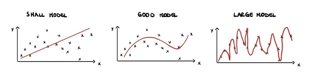
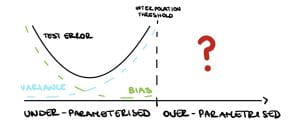
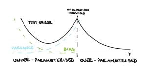
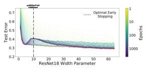
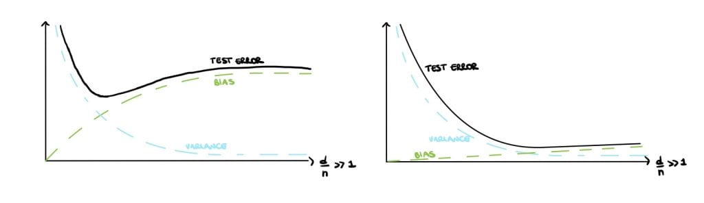
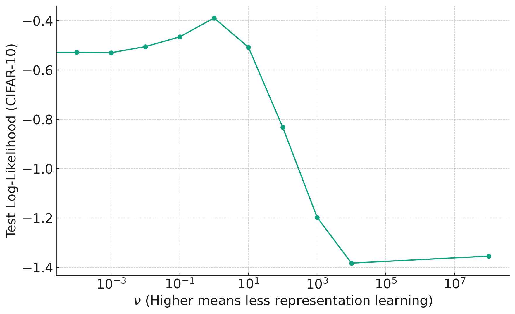
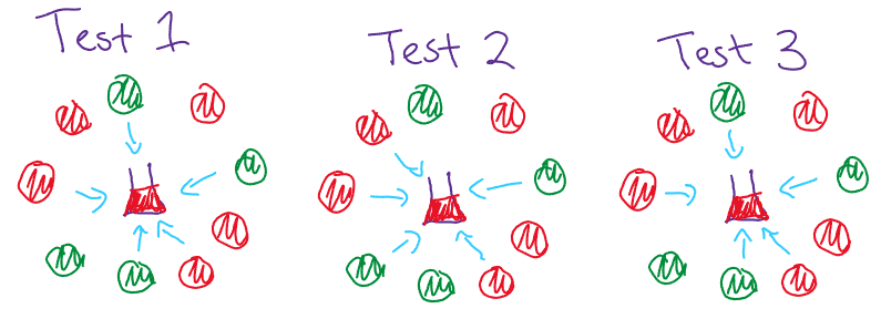
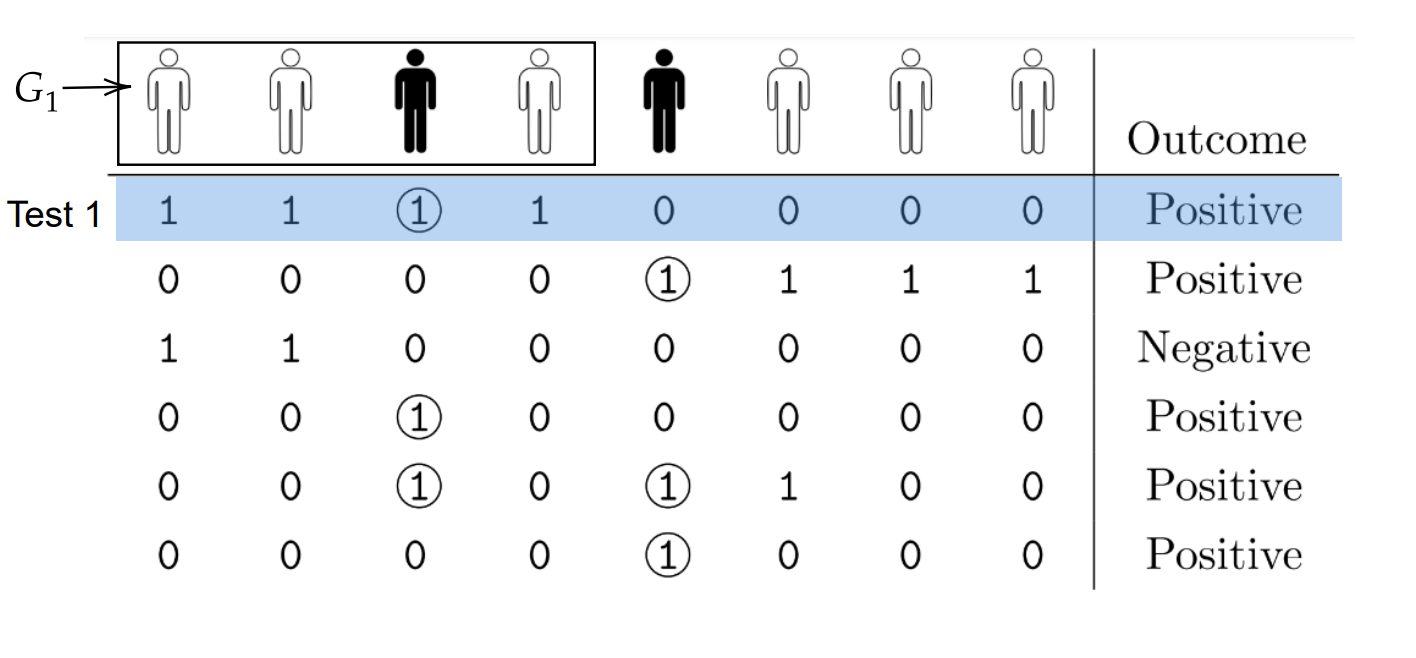
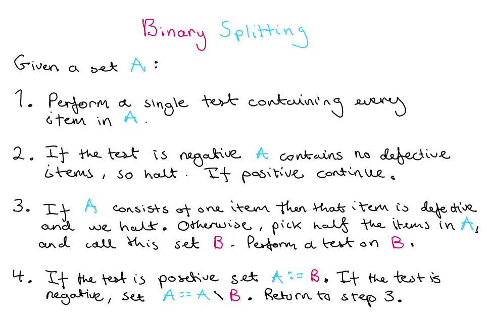
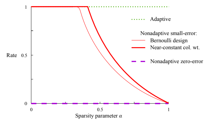 A graph comparing different group testing designs, where the $\text{Rate} = \log_2\binom{n}{k}/T$ where $T$ is the number of tests needed to recover all the defective items (with high probability for the red lines and with certainty for the purple line). [1]