Student Perspectives: Impurity Identification in Oligonucleotide Drug Samples

A post by Harry Tata, PhD student on the Compass programme.

Oligonucleotides in Medicine

Oligonucleotide therapies are at the forefront of modern pharmaceutical research and development, with recent years seeing major advances in treatments for a variety of conditions. Oligonucleotide drugs for Duchenne muscular dystrophy (FDA approved) [1], Huntington’s disease (Phase 3 clinical trials) [2], and Alzheimer’s disease [3] and amyotrophic lateral sclerosis (early-phase clinical trials) [4] show their potential for tackling debilitating and otherwise hard-to-treat conditions. With continuing development of synthetic oligonucleotides, analytical techniques such as mass spectrometry must be tailored to these molecules and keep pace with the field.

Working in conjunction with AstraZeneca, this project aims to advance methods for impurity detection and quantification in synthetic oligonucleotide mass spectra. In this blog post we apply a regularised version of the Richardson-Lucy algorithm, an established technique for image deconvolution, to oligonucleotide mass spectrometry data. This allows us to attribute signals in the data to specific molecular fragments, and therefore to detect impurities in oligonucleotide synthesis.

Oligonucleotide Fragmentation

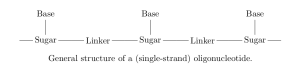
If we have attempted to synthesise an oligonucleotide \mathcal O with a particular sequence, we can take a sample from this synthesis and analyse it via mass spectrometry. In this process, molecules in the sample are first fragmented — broken apart into ions — and these charged fragments are then passed through an electromagnetic field. The trajectory of each fragment through this field depends on its mass/charge ratio (m/z), so measuring these trajectories (e.g. by measuring time of flight before hitting some detector) allows us to calculate the m/z of fragments in the sample. This gives us a discrete mass spectrum: counts of detected fragments (intensity) across a range of m/z bins [5].

To get an idea of how much of \mathcal O is in a sample, and what impurities might be present, we first need to consider what fragments \mathcal O will produce. Oligonucleotides are short strands of DNA or RNA; polymers with a backbone of sugars (such as ribose in RNA) connected by linkers (e.g. a phosphodiester bond), where each sugar has an attached base which encodes genetic information [6].

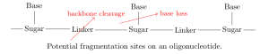
On each monomer, there are two sites where fragmentation is likely to occur: at the linker (backbone cleavage) or between the base and sugar (base loss). Specifically, depending on which bond within the linker is broken, there are four modes of backbone cleavage [7,8].
We include in \mathcal F every product of a single fragmentation of \mathcal O — any of the four backbone cleavage modes or base loss anywhere along the nucleotide — as well as the results of every combination of two fragmentations (different cleavage modes at the same linker are mutually exclusive).

Sparse Richardson-Lucy Algorithm

Suppose we have a chemical sample which we have fragmented and analysed by mass spectrometry. This gives us a spectrum across n bins (each bin corresponding to a small m/z range), and we represent this spectrum with the column vector \mathbf{b}\in\mathbb R^n, where b_i is the intensity in the i^{th} bin. For a set \{f_1,\ldots,f_m\}=\mathcal F of possible fragments, let x_j be the amount of f_j that is actually present. We would like to estimate the amounts of each fragment based on the spectrum \mathbf b.

If we had a sample comprising a unit amount of a single fragment f_j, so x_j=1 and x_{k\ne j}=0, and this produced a spectrum \begin{pmatrix}a_{1j}&\ldots&a_{nj}\end{pmatrix}^T, we can say the intensity contributed to bin i by x_j is a_{ij}. In mass spectrometry, the intensity in a single bin due to a single fragment is linear in the amount of that fragment, and the intensities in a single bin due to different fragments are additive, so in some general spectrum we have b_i=\sum_j x_ja_{ij}.

By constructing a library matrix \mathbf{A}\in\mathbb R^{n\times m} such that \{\mathbf A\}_{ij}=a_{ij} (so the columns of \mathbf A correspond to fragments in \mathcal F), then in ideal conditions the vector of fragment amounts \mathbf x=\begin{pmatrix}x_1&\ldots&x_m\end{pmatrix}^T solves \mathbf{Ax}=\mathbf{b}. In practice this exact solution is not found — due to experimental noise and potentially because there are contaminant fragments in the sample not included in \mathcal F — and we instead make an estimate \mathbf {\hat x} for which \mathbf{A\hat x} is close to \mathbf b.

Note that the columns of \mathbf A correspond to fragments in \mathcal F: the values in a single column represent intensities in each bin due to a single fragment only. We \ell_1-normalise these columns, meaning the total intensity (over all bins) of each fragment in the library matrix is uniform, and so the values in \mathbf{\hat x} can be directly interpreted as relative abundances of each fragment.

The observed intensities — as counts of fragments incident on each bin — are realisations of latent Poisson random variables. Assuming these variables are i.i.d., it can be shown that the estimate of \mathbf{x} which maximises the likelihood of the system is approximated by the iterative formula

\mathbf {\hat{x}}^{(t+1)}=\left(\mathbf A^T \frac{\mathbf b}{\mathbf{A\hat x}^{(t)}}\right)\odot \mathbf{\hat x}^{(t)}.

Here, quotients and the operator \odot represent (respectively) elementwise division and multiplication of two vectors. This is known as the Richardson-Lucy algorithm [9].

In practice, when we enumerate oligonucleotide fragments to include in \mathcal F, most of these fragments will not actually be produced when the oligonucleotide passes through a mass spectrometer; there is a large space of possible fragments and (beyond knowing what the general fragmentation sites are) no well-established theory allowing us to predict, for a new oligonucleotide, which fragments will be abundant or negligible. This means we seek a sparse estimate, where most fragment abundances are zero.

The Richardson-Lucy algorithm, as a maximum likelihood estimate for Poisson variables, is analagous to ordinary least squares regression for Gaussian variables. Likewise lasso regression — a regularised least squares regression which favours sparse estimates, interpretable as a maximum a posteriori estimate with Laplace priors — has an analogue in the sparse Richardson-Lucy algorithm:

\mathbf {\hat{x}}^{(t+1)}=\left(\mathbf A^T \frac{\mathbf b}{\mathbf{A\hat x}^{(t)}}\right)\odot \frac{ \mathbf{\hat x}^{(t)}}{\mathbf 1 + \lambda},

where \lambda is a regularisation parameter [10].

Library Generation

For each oligonucleotide fragment f\in\mathcal F, we smooth and bin the m/z values of the most abundant isotopes of f, and store these values in the columns of \mathbf A. However, if these are the only fragments in \mathcal F then impurities will not be identified: the sparse Richardson-Lucy algorithm will try to fit oligonucleotide fragments to every peak in the spectrum, even ones that correspond to fragments not from the target oligonucleotide. Therefore we also include ‘dummy’ fragments corresponding to single peaks in the spectrum — the method will fit these to non-oligonucleotide peaks, showing the locations of any impurities.

Results

For a mass spectrum from a sample containing a synthetic oligonucleotide, we generated a library of oligonucleotide and dummy fragments as described above, and applied the sparse Richardson-Lucy algorithm. Below, the model fit is plotted alongside the (smoothed, binned) spectrum and the ten most abundant fragments as estimated by the model. These fragments are represented as bars with binned m/z at the peak fragment intensity, and are separated into oligonucleotide fragments and dummy fragments indicating possible impurities. All intensities and abundances are Anscombe transformed (x\rightarrow\sqrt{x+3/8}) for clarity.

As the oligonucleotide in question is proprietary, its specific composition and fragmentation is not mentioned here, and the bins plotted have been transformed (without changing the shape of the data) so that individual fragment m/z values are not identifiable.

We see the data is fit extremely closely, and that the spectrum is quite clean: there is one very pronounced peak roughly in the middle of the m/z range. This peak corresponds to one of the oligonucleotide fragments in the library, although there is also an abundant dummy fragment slightly to the left inside the main peak. Fragment intensities in the library matrix are smoothed, and it may be the case that the smoothing here is inappropriate for the observed peak, hence other fragments being fit at the peak edge. Investigating these effects is a target for the rest of the project.

We also see several smaller peaks, most of which are modelled with oligonucleotide fragments. One of these peaks, at approximately bin 5352, has a noticeably worse fit if excluding dummy fragments from the library matrix (see below). Using dummy fragments improves this fit and indicates a possible impurity. Going forward, understanding and quantification of these impurities will be improved by including other common fragments in the library matrix, and by grouping fragments which correspond to the same molecules.

References

[1] Junetsu Igarashi, Yasuharu Niwa, and Daisuke Sugiyama. “Research and Development of Oligonucleotide Therapeutics in Japan for Rare Diseases”. In: Future Rare Diseases 2.1 (Mar. 2022), FRD19.

[2] Karishma Dhuri et al. “Antisense Oligonucleotides: An Emerging Area in Drug Discovery and Development”. In: Journal of Clinical Medicine 9.6 (6 June 2020), p. 2004.

[3] Catherine J. Mummery et al. “Tau-Targeting Antisense Oligonucleotide MAPTRx in Mild Alzheimer’s Disease: A Phase 1b, Randomized, Placebo-Controlled Trial”. In: Nature Medicine (Apr. 24, 2023), pp. 1–11.

[4] Benjamin D. Boros et al. “Antisense Oligonucleotides for the Study and Treatment of ALS”. In: Neurotherapeutics: The Journal of the American Society for Experimental NeuroTherapeutics 19.4 (July 2022), pp. 1145–1158.

[5] Ingvar Eidhammer et al. Computational Methods for Mass Spectrometry Proteomics. John Wiley & Sons, Feb. 28, 2008. 299 pp.

[6] Harri Lönnberg. Chemistry of Nucleic Acids. De Gruyter, Aug. 10, 2020.

[7] S. A. McLuckey, G. J. Van Berkel, and G. L. Glish. “Tandem Mass Spectrometry of Small, Multiply Charged Oligonucleotides”. In: Journal of the American Society for Mass Spectrometry 3.1 (Jan. 1992), pp. 60–70.

[8] Scott A. McLuckey and Sohrab Habibi-Goudarzi. “Decompositions of Multiply Charged Oligonucleotide Anions”. In: Journal of the American Chemical Society 115.25 (Dec. 1, 1993), pp. 12085–12095.

[9] Mario Bertero, Patrizia Boccacci, and Valeria Ruggiero. Inverse Imaging with Poisson Data: From Cells to Galaxies. IOP Publishing, Dec. 1, 2018.

[10] Elad Shaked, Sudipto Dolui, and Oleg V. Michailovich. “Regularized Richardson-Lucy Algorithm for Reconstruction of Poissonian Medical Images”. In: 2011 IEEE International Symposium on Biomedical Imaging: From Nano to Macro. Mar. 2011, pp. 1754–1757.


Compass students attending AISTATS 2023 in Valencia

We (Ed Davis, Josh Givens, Alex Modell, and Hannah Sansford) attended the 2023 AISTATS conference in Valencia in order to explore the interesting research being presented as well as present some of our own work. While we talked about our work being published at the conference in this earlier blog post, having now attended the conference, we thought we’d talk about our experience there. We’ll spotlight some of the talks and posters which interested us most and talk about our highlights of Valencia as a whole.

Talks & Posters

Mode-Seeking Divergences: Theory and Applications to GANs

One especially interesting talk and poster at the conference was presented by Cheuk Ting Li on their work in collaboration with Farzan Farnia. This work aims to set up a formal classification for various probability measure divergences (such as f-Divergences, Wasserstein distance, etc.) in terms of there mode-seeking or mode-covering properties. By mode-seeking/mode-covering we mean the behaviour of the divergence when used to fit a unimodal distribution to a multi-model target. Specifically a mode-seeking divergence will encourage the target distribution to fit just one of the modes ignoring the other while a mode covering divergence will encourage the distribution to cover all modes leading to less accurate fitting on an individual mode but better covering the full support of the distribution. While these notions of mode-seeking and mode-covering divergences had been discussed before, up to this point there seems to be no formal definition for these properties, and disagreement on the appropriate categorisation of some divergences. This work presents such a definition and uses it to categorise many of the popular divergence methods. Additionally they show how an additive combination a mode seeking f-divergence and the 1-Wasserstein distance retain the mode-seeking property of the f-divergence while being implementable using only samples from our target distribution (rather than knowledge of the distribution itself) making it a desirable divergence for use with GANs.

Talk: https://youtu.be/F7LdHIzZQow

Paper: https://proceedings.mlr.press/v206/ting-li23a.html

Using Sliced Mutual Information to Study Memorization and Generalization in
Deep Neural Networks

The benefit of attending large conferences like AISTATS is having the opportunity to hear talks that are not related to your main research topic. This was the case with a talk by Wongso et. al. was one such talk. Although it did not overlap with any of our main research areas, we all found this talk very interesting.
The talk was on the topic of tracking memorisation and generalisation in deep neural networks (DNNs) through the use of /sliced mutual information/. Mutual information (MI) is commonly used in information theory and represents the reduction of uncertainty about one random variable, given the knowledge of the other. However, MI is hard to estimate in high dimensions, which makes it a prohibitive metric for use in neural networks.
Enter sliced mutual information (SMI). This metric is the average of the MI terms between their one-dimensional projections. The main difference between SMI and MI is that SMI is scalable to high dimensions and scales faster than MI.
Next, let’s talk about memorisation. Memorisation is known to occur in DNNs and is where the DNN fits random labels in training as it has memorised noisy labels in training, leading to bad generalisation. The authors demonstrate this behaviour by fitting a multi-layer perceptron to the MNIST dataset with various amounts of label noise. As the noise increased, the difference between the training and test accuracy became greater.
As the label noise increases, the MI between the features and target variable does not change, meaning that MI did not track the loss in generalisation. However, the authors show that the SMI did track the generalisation. As the label noise increased, the SMI decreased significantly as the MLP’s generalisation got worse. Their main theorem showed that SMI is lower-bounded by a term which includes the spherical soft-margin separation, a quantity which is used to track memorisation and generalisation!
In summary, unlike MI, SMI can track memorization and generalisation in DNNs. If you’d like to know more, you can find the full paper here: https://proceedings.mlr.press/v206/wongso23a.html.

Invited Speakers and the Test of Time Award

As well as the talks on papers that had been selected for oral presentation, each day began with a (longer) invited talk which, for many of us, were highlights of each day. The invited speakers were extremely engaging and covered varied and interesting topics; from Arthur Gretton (UCL) presenting ‘Causal Effect Estimation with Context and Confounders’ to Shakir Mohamed (DeepMind) presenting ‘Elevating our Evaluations: Technical and Sociotechnical Standards of Assessment in Machine Learning’. A favourite amongst us was a talk from Tamara Broderick (MIT) titled ‘An Automatic Finite-Sample Robustness Check: Can Dropping a Little Data Change Conclusions?’. In this talk she addressed a worry that researchers might have when the goal is to analyse a data sample and apply any conclusions to a new population: was a small proportion of the data sample instrumental to the original conclusion? Tamara and collorators propose a method to assess the sensitivity of statistical conclusions to the removal of a very small fraction of the data set. They find that sensitivity is driven by a signal-to-noise ratio in the inference problem, does not disappear asymptotically, and is not decided by misspecification. In experiments they find that many data analyses are robust, but that the conclusions of severeal influential economics papers can be changed by removing (much) less than 1% of the data! A link to the talk can be found here: https://youtu.be/QYtIEqlwLHE

This year, AISTATS featured a Test of Time Award to recognise a paper from 10 years ago that has had a prominent impact in the field. It was awarded to Andreas Damianou and Neil Lawrence for the paper ‘Deep Gaussian Processes’, and their talk was a definite highlight of the conferece. Many of us had seen Neil speak at a seminar at the University of Bristol last year and, being the engaging speaker he is, we were looking forward to hearing him speak again. Rather than focussing on the technical details of the paper, Neils talk concentrated on his (and the machine learning community’s) research philosophy in the years preceeding writing the paper, and how the paper came about – a very interesting insight, and a refreshing break from the many technical talks!

Valencia

There was so much to like about Valencia even from our short stay there. We’ll try and give you a very brief highlight of our favourite things.

Food & Drink:

Obviously Valencia is renowned for being the birthplace of paella and while the paella was good we sampled many other delights our stay. Our collective highlight was the nicest Burrata any of us had ever had which, in a stunning display of individualism, all four of us decided to get on our first day at the conference.

Artist rendition of our 4 meals.

Beach:

About half an hours tram ride from the conference centre are the beaches of Valencia. These stretch for miles as well as having a good 100m in depth with (surprisingly hot) sand covering the lot. We visited these after the end of the conference on the Thursday and despite it being the only cloudy day of the week it was a perfect way to relax at the end of a hectic few days with the pleasantly temperate water being an added bonus.

Architecture:

Valencia has so much interesting architecture scattered around the city centre. One of the most memorable remarkable places was the San Nicolás de Bari and San Pedro Mártir (Church of San Nicolás) which is known as the Sistine chapel of Valencia (according to the audio-guide for the church at least) with its incredible painted ceiling and live organ playing.

Ceiling of the Church of San Nicolás


Student Perspectives: Intro to Recommendation Systems

A post by Hannah Sansford, PhD student on the Compass programme.

Introduction

Like many others, I interact with recommendation systems on a daily basis; from which toaster to buy on Amazon, to which hotel to book on booking.com, to which song to add to a playlist on Spotify. They are everywhere. But what is really going on behind the scenes?

Recommendation systems broadly fit into two main categories:

1) Content-based filtering. This approach uses the similarity between items to recommend items similar to what the user already likes. For instance, if Ed watches two hair tutorial videos, the system can recommend more hair tutorials to Ed.

2) Collaborative filtering. This approach uses the the similarity between users’ past behaviour to provide recommendations. So, if Ed has watched similar videos to Ben in the past, and Ben likes a cute cat video, then the system can recommend the cute cat video to Ed (even if Ed hasn’t seen any cute cat videos).

Both systems aim to map each item and each user to an embedding vector in a common low-dimensional embedding space E = \mathbb{R}^d. That is, the dimension of the embeddings (d) is much smaller than the number of items or users. The hope is that the position of these embeddings captures some of the latent (hidden) structure of the items/users, and so similar items end up ‘close together’ in the embedding space. What is meant by being ‘close’ may be specified by some similarity measure.

Collaborative filtering

In this blog post we will focus on the collaborative filtering system. We can break it down further depending on the type of data we have:

1) Explicit feedback data: aims to model relationships using explicit data such as user-item (numerical) ratings.

2) Implicit feedback data: analyses relationships using implicit signals such as clicks, page views, purchases, or music streaming play counts. This approach makes the assumption that: if a user listens to a song, for example, they must like it.

The majority of the data on the web comes from implicit feedback data, hence there is a strong demand for recommendation systems that take this form of data as input. Furthermore, this form of data can be collected at a much larger scale and without the need for users to provide any extra input. The rest of this blog post will assume we are working with implicit feedback data.

Problem Setup

Suppose we have a group of n users U = (u_1, \ldots, u_n) and a group of m items I = (i_1, \ldots, i_m). Then we let \mathbf{R} \in \mathbb{R}^{n \times m} be the ratings matrix where position R_{ui} represents whether user u interacts with item i. Note that, in most cases the matrix \mathbf{R} is very sparse, since most users only interact with a small subset of the full item set I. For any items i that user u does not interact with, we set R_{ui} equal to zero. To be clear, a value of zero does not imply the user does not like the item, but that they have not interacted with it. The final goal of the recommendation system is to find the best recommendations for each user of items they have not yet interacted with.

Matrix Factorisation (MF)

A simple model for finding user emdeddings, \mathbf{X} \in \mathbb{R}^{n \times d}, and item embeddings, \mathbf{Y} \in \mathbb{R}^{m \times d}, is Matrix Factorisation. The idea is to find low-rank embeddings such that the product \mathbf{XY}^\top is a good approximation to the ratings matrix \mathbf{R} by minimising some loss function on the known ratings.

A natural loss function to use would be the squared loss, i.e.

L(\mathbf{X}, \mathbf{Y}) = \sum_{u, i} \left(R_{ui} - \langle X_u, Y_i \rangle \right)^2.

This corresponds to minimising the Frobenius distance between \mathbf{R} and its approximation \mathbf{XY}^\top, and can be solved easily using the singular value decomposition \mathbf{R} = \mathbf{U S V}^\top.

Once we have our embeddings \mathbf{X} and \mathbf{Y}, we can look at the row of \mathbf{XY}^\top corresponding to user u and recommend the items corresponding to the highest values (that they haven’t already interacted with).

Logistic MF

Minimising the loss function in the previous section is equivalent to modelling the probability that user u interacts with item i as the inner product \langle X_u, Y_i \rangle, i.e.

R_{ui} \sim \text{Bernoulli}(\langle X_u, Y_i \rangle),

and maximising the likelihood over \mathbf{X} and \mathbf{Y}.

In a research paper from Spotify [3], this relationship is instead modelled according to a logistic function parameterised by the sum of the inner product above and user and item bias terms, \beta_u and \beta_i,

R_{ui} \sim \text{Bernoulli} \left( \frac{\exp(\langle X_u, Y_i \rangle + \beta_u + \beta_i)}{1 + \exp(\langle X_u, Y_i \rangle + \beta_u + \beta_i)} \right).

Relation to my research

A recent influential paper [1] proved an impossibility result for modelling certain properties of networks using a low-dimensional inner product model. In my 2023 AISTATS publication [2] we show that using a kernel, such as the logistic one in the previous section, to model probabilities we can capture these properties with embeddings lying on a low-dimensional manifold embedded in infinite-dimensional space. This has various implications, and could explain part of the success of Spotify’s logistic kernel in producing good recommendations.

References

[1] Seshadhri, C., Sharma, A., Stolman, A., and Goel, A. (2020). The impossibility of low-rank representations for triangle-rich complex networks. Proceedings of the National Academy of Sciences, 117(11):5631–5637.

[2] Sansford, H., Modell, A., Whiteley, N., and Rubin-Delanchy, P. (2023). Implications of sparsity and high triangle density for graph representation learning. Proceedings of The 26th International Conference on Artificial Intelligence and Statistics, PMLR 206:5449-5473.

[3] Johnson, C. C. (2014). Logistic matrix factorization for implicit feedback data. Advances in Neural Information Processing Systems, 27(78):1–9.


Compass students attending the Workshop on Functional Inference and Machine Intelligence (FIMI) at ISM Tokyo

A post by Compass CDT students Edward Milsom, Jake Spiteri, Jack Simons, and Sam Stockman.

We (Edward Milsom, Jake Spiteri, Jack Simons, Sam Stockman) attended the 2023 Workshop on Functional Inference and Machine Intelligence (FIMI) taking place on the 14, 15 and 16th of March at the Institute of Statistical Mathematics in Tokyo, Japan. Our attendance to the workshop was to further collaborative ties between the two institutions. The in-person participants included many distinguished academics from around Japan as well as our very own Dr Song Liu. Due to the workshops modest size, there was an intimate atmosphere which nurtured many productive research discussions. Whilst staying in Tokyo, we inevitably sampled some Japanese culture, from Izakayas to cherry blossoms and sumo wrestling!

We thought we’d share some of our thoughts and experiences. We’ll first go through some of our most memorable talks, and then talk about some of our activities outside the workshop.

Talks

Sho Sonoda – Ridgelet Transforms for Neural Networks on Manifolds and Hilbert Spaces

We particularly enjoyed the talk given by Sho Sonoda, a Research Scientist from the Deep Learning Theory group at Riken AIP on “Ridgelet Transforms for Neural Networks on Manifolds and Hilbert Spaces.” Sonoda’s research aims to demystify the black box nature of neural networks, shedding light on how they work and their universal approximation capabilities. His talk provided valuable insights into the integral representations of neural networks, and how they can be represented using ridgelet transforms. Sonoda presented a reconstruction formula from which we see that if a neural network can be represented using ridgelet transforms, then it is a universal approximator. He went on to demonstrate that various types of networks, such as those on finite fields, group convolutional neural networks (GCNNs), and networks on manifolds and Hilbert spaces, can be represented in this manner and are thus universal approximators. Sonoda’s work improves upon existing universality theorems by providing a more unified and direct approach, as opposed to the previous case-by-case methods that relied on manual adjustments of network parameters or indirect conversions of (G)CNNs into other universal approximators, such as invariant polynomials and fully-connected networks. Sonoda’s work is an important step toward a more transparent and comprehensive understanding of neural networks.

Greg Yang – The unreasonable effectiveness of mathematics in large scale deep learning

Greg Yang is a researcher at Microsoft Research who is working on a framework for understanding neural networks called “tensor programs”. Similar to Neural Tangent Kernels and Neural Network Gaussian Processes, the tensor program framework allows us to consider neural networks in the infinite-width limit, where it becomes possible to make statements about the properties of very wide networks. However, tensor programs aim to unify existing work on infinite-width neural networks by allowing one to take the infinite limit of a much wider range of neural network architectures using one single framework.

In his talk, Yang discussed his most recent work in this area, concerning the “maximal update parametrisation”. In short, they show that in this parametrisation, the optimal hyperparameters of very wide neural networks are the same as those for much smaller neural networks. This means that hyperparameter search can be done using small, cheap models, and then applied to very large models like GPT-3, where hyperparameter search would be too expensive. The result is summarised in this figure from their paper “Tensor Programs V: Tuning Large Neural Networks via Zero-Shot Hyperparameter Transfer”, which shows how this is not possible in the standard parametrisation. This work was only possible by building upon the tensor program framework, thereby demonstrating the value of having a solid theoretical understanding of neural networks.

Statistical Seismology Seminar Series

In addition to the workshop, Sam attended the 88th Statistical Seismology seminar in the Risk Analysis Research Centre at ISM https://www.ism.ac.jp/~ogata/Ssg/ssg_statsei_seminarsE.html. The Statistical Seismology Research Group at ISM was created by Emeritus Professor Yosihiko Ogata and is one of the leading global research institutes for statistical seismology. Its most significant output has been the Epidemic-Type Aftershock Sequence (ETAS) model, a point process based earthquake forecasting model that has been the most dominant model for forecasting since its creation by Ogata in 1988.

As part of the Seminar series, Sam gave a talk on his most recent work (Forecasting the 2016-2017 Central Apennines Earthquake Sequence with a Neural Point Process’, https://arxiv.org/abs/2301.09948) to the research group and other visiting academics.

Japan’s interest is earthquake science is due to the fact that they record the most earthquakes in the world. The whole country is in a very active seismic area, and they have the densest seismic network. So even though they might not actually have the most earthquakes in the world (which is most likely Indonesia) they certainly document the most. The evening before flying back to the UK, Sam and Jack felt a magnitude 5.2 earthquake 300km north of Tokyo in the Miyagi prefecture. At that distance all that was felt was a small shudder…

Japan

It’s safe to say that the abundance of delicious food was the most memorable aspect of our trip. In fact, we never had a bad meal! Our taste buds were taken on a culinary journey as we tried a variety of Japanese dishes. From hearty, broth-based bowls of ramen and tsukemen, to fun conveyor-belt sushi restaurants, and satisfying tonkatsu (breaded deep-fried pork cutlet) with sticky rice or spicy udon noodles, we were never at a loss for delicious options. We even had the opportunity to cook our own food at an indoor barbecue!

Aside from the food, we thoroughly enjoyed our time in Tokyo – exploring the array of second-hand clothes shops, relaxing in bath-houses, and trying random things from the abundance of vending machines.


Compass students at AISTATS 2023

Congratulations to Compass students Josh Givens, Hannah Sansford and Alex Modell who, along with their supervisors have had their papers accepted to be published at AISTATS 2023.


‘Implications of sparsity and high triangle density for graph representation learning’

Hannah Sansford, Alexander Modell, Nick Whiteley, Patrick Rubin-Delanchy

Hannah: In this paper we explore the implications of two common characteristics of real-world networks, sparsity and triangle-density, for graph representation learning. An example of where these properties arise in the real-world is in social networks, where, although the number of connections each individual has compared to the size of the network is small (sparsity), often a friend of a friend is also a friend (triangle-density). Our result counters a recent influential paper that shows the impossibility of simultaneously recovering these properties with finite-dimensional representations of the nodes, when the probability of connection is modelled by the inner-product. We, by contrast, show that it is possible to recover these properties using an infinite-dimensional inner-product model, where representations lie on a low-dimensional manifold. One of the implications of this work is that we can ‘zoom-in’ to local neighbourhoods of the network, where a lower-dimensional representation is possible.

The paper has been selected for oral presentation at the conference in Valencia (<2% of submissions). 


Density Ratio Estimation and Neyman Pearson Classification with Missing Data

Josh Givens, Song Liu, Henry W J Reeve

Josh: In our paper we adapt the popular density ratio estimation procedure KLIEP to make it robust to missing not at random (MNAR) data and demonstrate its efficacy in Neyman-Pearson (NP) classification. Density ratio estimation (DRE) aims to characterise the difference between two classes of data by estimating the ratio between their probability densities. The density ratio is a fundamental quantity in statistics appearing in many settings such as classification, GANs, and covariate shift making its estimation a valuable goal. To our knowledge there is no prior research into DRE with MNAR data, a missing data paradigm where the likelihood of an observation being missing depends on its underlying value. We propose the estimator M-KLIEP and provide finite sample bounds on its accuracy which we show to be minimax optimal for MNAR data. To demonstrate the utility of this estimator we apply it the the field of NP classification. In NP classification we aim to create a classifier which strictly controls the probability of incorrectly classifying points from one class. This is useful in any setting where misclassification for one class is much worse than the other such as fault detection on a production line where you would want to strictly control the probability of classifying a faulty item as non-faulty. In addition to showing the efficacy of our new estimator in this setting we also provide an adaptation to NP classification which allows it to still control this misclassification probability even when fit using MNAR data.

Student Perspectives: An Introduction to Stochastic Gradient Methods

A post by Ettore Fincato, PhD student on the Compass programme.

This post provides an introduction to Gradient Methods in Stochastic Optimisation. This class of algorithms is the foundation of my current research work with Prof. Christophe Andrieu and Dr. Mathieu Gerber, and finds applications in a great variety of topics, such as regression estimation, support vector machines, convolutional neural networks.

We can see below a simulation by Emilien Dupont (https://emiliendupont.github.io/) which represents two trajectories of an optimisation process of a time-varying function. This well describes the main idea behind the algorithms we will be looking at, that is, using the (stochastic) gradient of a (random) function to iteratively reach the optimum.

Stochastic Optimisation

Stochastic optimisation was introduced by [1], and its aim is to find a scheme for solving equations of the form \nabla_w g(w)=0 given “noisy” measurements of g [2].

In the simplest deterministic framework, one can fully determine the analytical form of g(w), knows that it is differentiable and admits an unique minimum – hence the problem

w_*=\underset{w}{\text{argmin}}\quad g(w)

is well defined and solved by \nabla_w g(w)=0.

On the other hand, one may not be able to fully determine g(w) because his experiment is corrupted by a random noise. In such cases, it is common to identify this noise with a random variable, say V, consider an unbiased estimator \eta(w,V) s.t. \mathbb{E}_V[\eta(w,V)]=g(w) and to rewrite the problem as

w_*=\underset{w}{\text{argmin}}\quad\mathbb{E}_V[\eta(w,V)].

(more…)

Student Perspectives: An Introduction to Deep Kernel Machines

A post by Edward Milsom, PhD student on the Compass programme.

This blog post provides a simple introduction to Deep Kernel Machines[1] (DKMs), a novel supervised learning method that combines the advantages of both deep learning and kernel methods. This work provides the foundation of my current research on convolutional DKMs, which is supervised by Dr Laurence Aitchison.

Why aren’t kernels cool anymore?

Kernel methods were once top-dog in machine learning due to their ability to implicitly map data to complicated feature spaces, where the problem usually becomes simpler, without ever explicitly computing the transformation. However, in the past decade deep learning has become the new king for complicated tasks like computer vision and natural language processing.

Neural networks are flexible when learning representations

The reason is twofold: First, neural networks have millions of tunable parameters that allow them to learn their feature mappings automatically from the data, which is crucial for domains like images which are too complex for us to specify good, useful features by hand. Second, their layer-wise structure means these mappings can be built up to increasingly more abstract representations, while each layer itself is relatively simple[2]. For example, trying to learn a single function that takes in pixels from pictures of animals and outputs their species is difficult; it is easier to map pixels to corners and edges, then shapes, then body parts, and so on.

Kernel methods are rigid when learning representations

It is therefore notable that classical kernel methods lack these characteristics: most kernels have a very small number of tunable hyperparameters, meaning their mappings cannot flexibly adapt to the task at hand, leaving us stuck with a feature space that, while complex, might be ill-suited to our problem. (more…)

Student perspectives: ensemble modelling for probabilistic volcanic ash hazard forecasting

A post by Shannon Williams, PhD student on the Compass programme.

My PhD focuses on the application of statistical methods to volcanic hazard forecasting. This research is jointly supervised by Professor Jeremy Philips (School of Earth Sciences) and Professor Anthony Lee. (more…)

Student perspectives: Neural Point Processes for Statistical Seismology

A post by Sam Stockman, PhD student on the Compass programme.

Introduction

Throughout my PhD I aim to bridge a gap between advances made in the machine learning community and the age-old problem of earthquake forecasting. In this cross-disciplinary work with Max Werner from the School of Earth Sciences and Dan Lawson from the School of Mathematics, I hope to create more powerful, efficient and robust models for forecasting, that can make earthquake prone areas safer for their inhabitants.

For years seismologists have sought to model the structure and dynamics of the earth in order to make predictions about earthquakes. They have mapped out the structure of fault lines and conducted experiments in the lab where they submit rock to great amounts of force in order to simulate plate tectonics on a small scale. Yet when trying to forecast earthquakes on a short time scale (that’s hours and days, not tens of years), these models based on the knowledge of the underlying physics are regularly outperformed by models that are statistically motivated. In statistical seismology we seek to make predictions through looking at distributions of the times, locations and magnitudes of earthquakes and use them to forecast the future.


(more…)

Student Perspectives: Application of Density Ratio Estimation to Likelihood-Free problems

A post by Jack Simons, PhD student on the Compass programme.

Introduction

I began my PhD with my supervisors, Dr Song Liu and Professor Mark Beaumont with the intention of combining their respective fields of research; Density Ratio Estimation (DRE), and Simulation Based Inference (SBI):

  • DRE is a rapidly growing paradigm in machine learning which (broadly) provides efficient methods of comparing densities without the need to compute each density individually. For a comprehensive yet accessible overview of DRE in Machine Learning see [1].
  • SBI is a group of methods which seek to solve Bayesian inference problems when the likelihood function is intractable. If you wish for a concise overview of the current work, as well as motivation then I recommend [2].

Last year we released a paper, Variational Likelihood-Free Gradient Descent [3] which combined these fields. This blog post seeks to condense, and make more accessible, the contents of the paper.

Motivation: Likelihood-Free Inference

Let’s begin by introducing likelihood-free inference. We wish to do inference on the posterior distribution of parameters \theta for a specific observation x=x_{\mathrm{obs}}, i.e. we wish to infer p(\theta|x_{\mathrm{obs}}) which can be decomposed via Bayes’ rule as

p(\theta|x_{\mathrm{obs}}) = \frac{p(x_{\mathrm{obs}}|\theta)p(\theta)}{\int p(x_{\mathrm{obs}}|\theta)p(\theta) \mathrm{d}\theta}.

The likelihood-free setting is that, additional to the usual intractability of the normalising constant in the denominator, the likelihood, p(x|\theta), is also intractable. In lieu of this, we require an implicit likelihood which describes the relation between data x and parameters \theta in the form of a forward model/simulator (hence simulation based inference!). (more…)

Skip to toolbar