
A post by Shannon Williams, PhD student on the Compass programme.
My PhD focuses on the application of statistical methods to volcanic hazard forecasting. This research is jointly supervised by Professor Jeremy Philips (School of Earth Sciences) and Professor Anthony Lee.
Introduction to probabilistic volcanic hazard forecasting
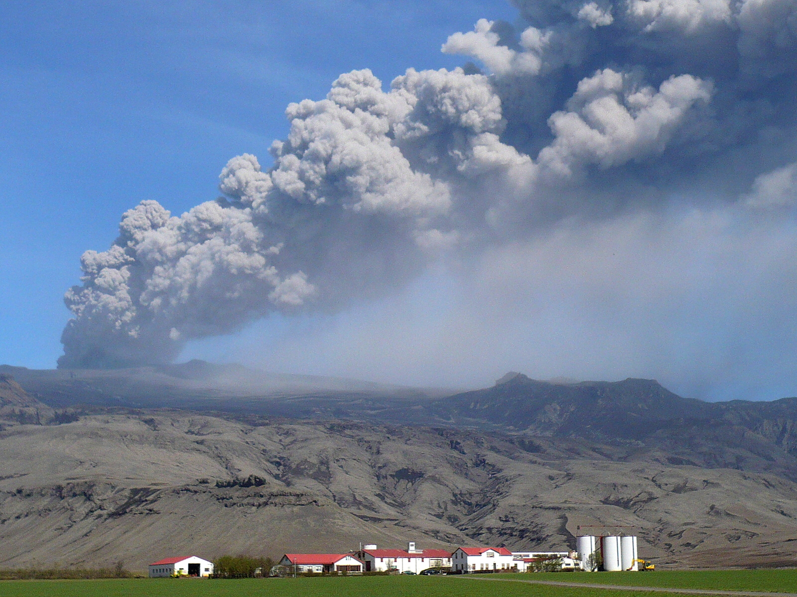
When an explosive volcanic eruption happens, large amounts of volcanic ash can be injected into the atmosphere and remain airborne for many hours to days from the onset of the eruption. Driven by atmospheric wind, this ash can travel up to thousands of kilometres downwind of the volcano and cause significant impacts on agriculture, infrastructure, and human health. Notably, a series of explosive eruptions from Eyjafjallajökull, Iceland between March and June 2010 resulted in the highest level of air travel disruption in Northern Europe since the Second World War, with the 108,000 flights cancelled and 1.7 billion USD in revenue lost.
The challenging task of forecasting volcanic ash dispersion is complicated by the chaotic nature of atmospheric wind fields and the lack of direct observations of ash concentration obtained during eruptive events.
Ensemble modelling
In order to construct probabilistic volcanic ash hazard assessments, volcanologists typically opt for an ensemble modelling approach in order to filter out the uncertainty in the meteorological conditions. This approach requires a model for the simulation of atmospheric ash dispersion, given eruption source conditions and meteorological inputs (referred to as forcing data). Typically a deterministic simulator such as FALL3D [1] is used, and so the uncertainty in the output is a direct consequence of the uncertainty in the inputs. To capture the uncertainty in the meteorological data, volcanologists construct an ensemble of simulations where the eruption conditions remain constant but the forcing data is altered, and average over the ensemble to produce an ash dispersion forecast [2].
Whilst this is a statistical approach by its construction and the objective is to provide probabilistic forecasts, predictions are often stated without providing a measure of the uncertainty in these predictions; furthermore, the ensemble size is typically decided on a pragmatic basis without consideration given to the magnitude of the probabilities of interest and the desired confidence in these probabilities. Much of my research since the beginning of my PhD has been on ways to enumerate these probabilities and their uncertainty, and on methods of deciding the ensemble size and reducing the uncertainty (variance) of the probability estimates.
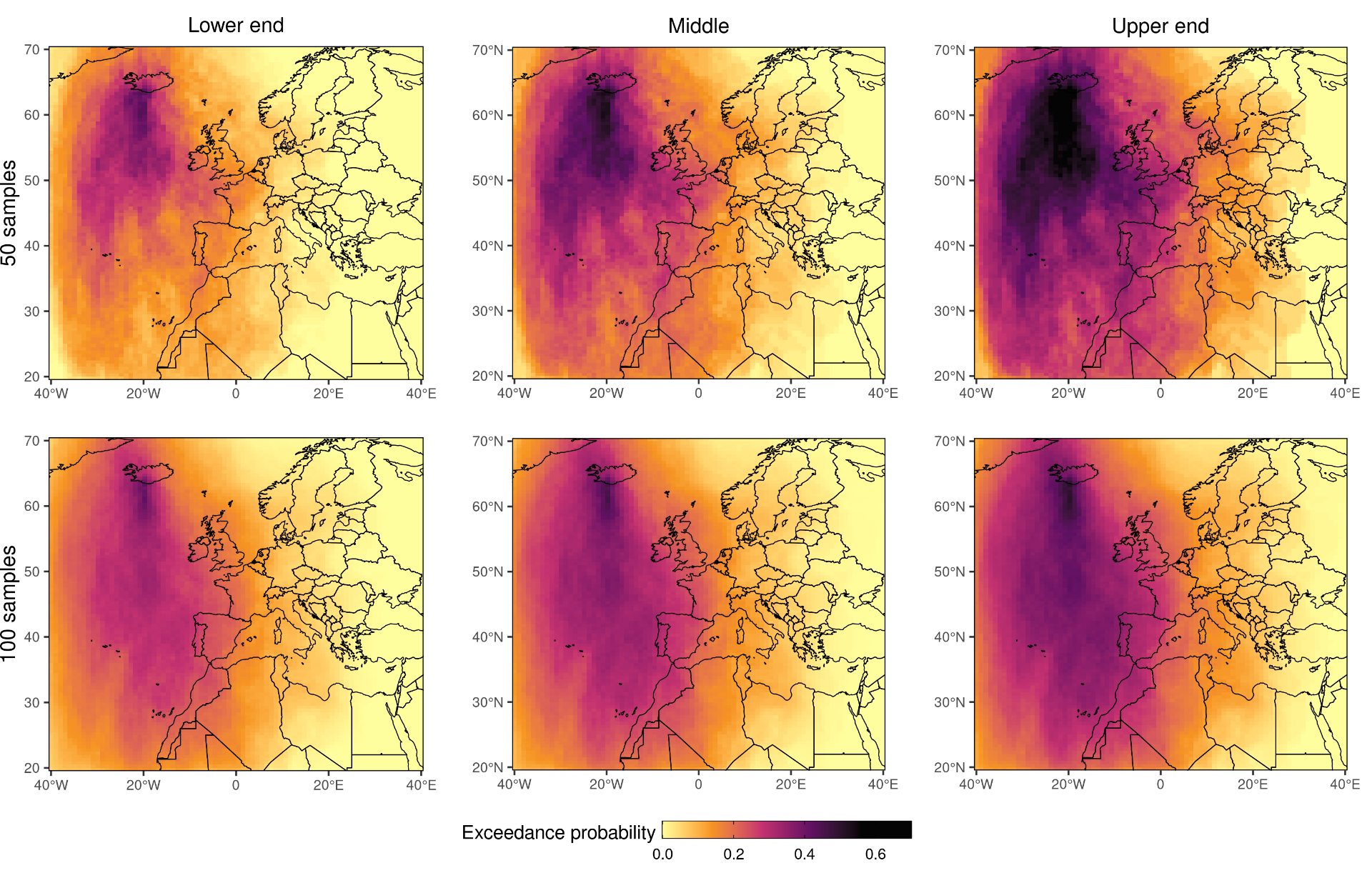
Ash concentration exceedance probabilities
A common exercise in volcanic ash hazard assessment is the computation of ash concentration exceedance probabilities [3]. Given an eruption scenario, which we provide to the model by defining inputs such as the volcanic plume height and the mass eruption rate, what is the probability that the ash concentration at some location exceeds a pre-defined threshold? For example, how likely is it that the ash concentration at some flight level near Heathrow airport exceeds 500 
Exceedance probability estimation
To construct an ensemble for exceedance probability estimation, we draw 


")

")

 \geq c\}")
where 


 = \mathbb{P}(\psi \circ \phi (Z_i) \geq c)")
representing the exceedance probability. As the ![\mathbb{E}[X_i]=p](https://s0.wp.com/latex.php?latex=%5Cmathbb%7BE%7D%5BX_i%5D%3Dp&bg=ffffff&fg=000000&s=0 "\mathbb{E}[X_i]=p")
 = p (1-p)")


which provides an unbiased estimate of
 = \frac{1}{n} p (1-p)")
Quantifying the uncertainty
This variance can be estimated by replacing 
}")
The figure below compares 95% confidence intervals for the probability of exceeding 500
 Commonly we would want to visualise estimates of probabilities of different magnitudes, corresponding to different thresholds, alongside each other. In this situation it is beneficial to view them on a logarithmic scale and provide confidence intervals for
 \pm 1.96 \sqrt{\frac{1-\hat{p}_n}{n \hat{p}_n}}")
The figure below illustrates exceedance probability estimates with 95% confidence intervals versus threshold for a number of locations in Europe on a double logarithmic scale, based on an ensemble size of 6000.
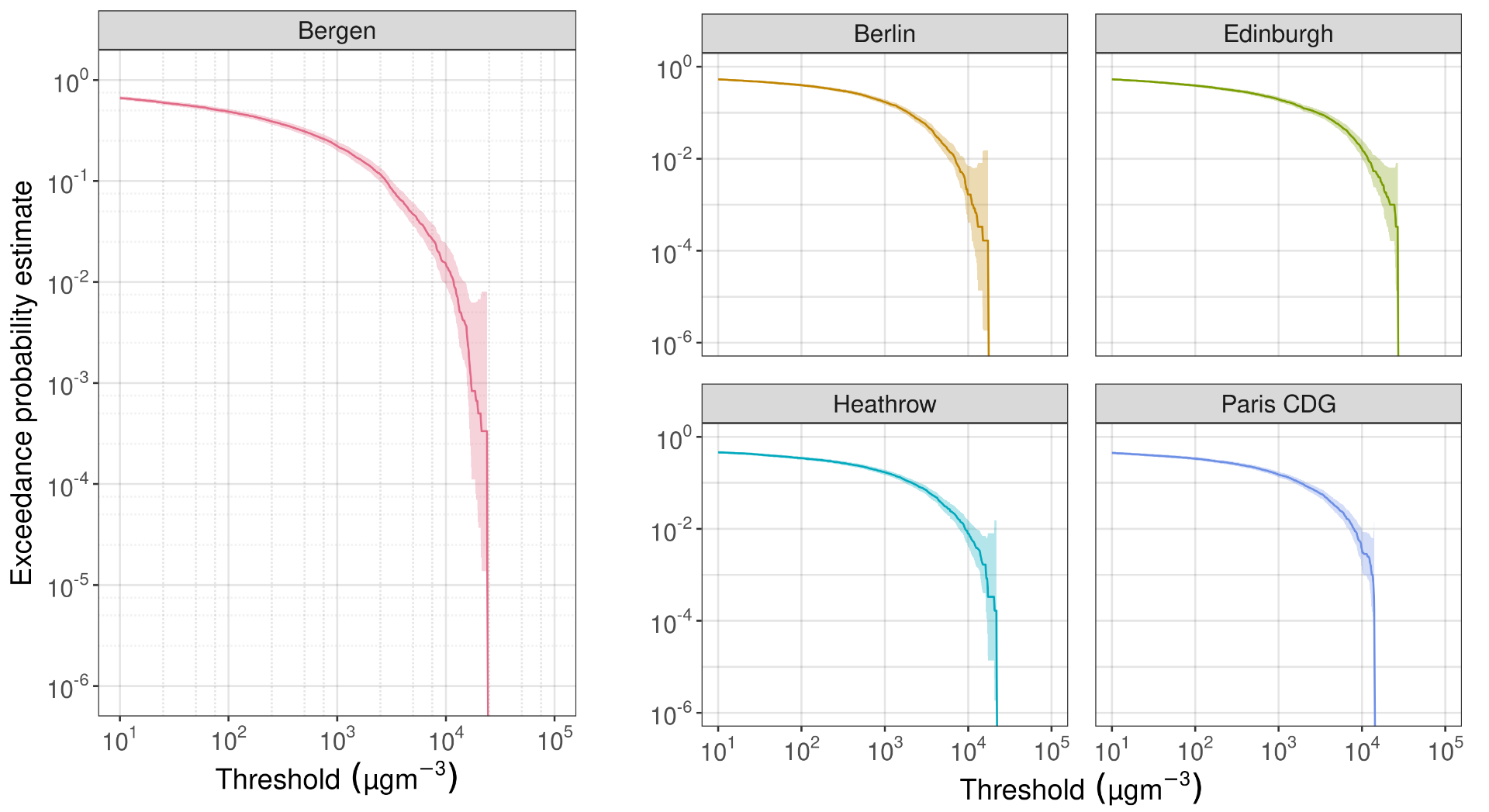
Choosing the ensemble size
Clearly, as the ash concentration threshold increases the probability of exceeding that threshold gets smaller. Fewer exceedance events will be seen in the ensemble than for lower thresholds, and the size of the confidence interval will be larger when compared with the magnitude of the probability itself.
It seems sensible to set the ensemble size based on the magnitude of the lowest probability of interest, and a natural way to do this is to consider the expected number of exceedances given
![\mathbb{E} \left[ \sum_{i=1}^n X_i \right] = \sum_{i=1}^n \mathbb{E} [X_i] = np](https://s0.wp.com/latex.php?latex=%5Cmathbb%7BE%7D+%5Cleft%5B+%5Csum_%7Bi%3D1%7D%5En+X_i+%5Cright%5D+%3D+%5Csum_%7Bi%3D1%7D%5En+%5Cmathbb%7BE%7D+%5BX_i%5D+%3D+np&bg=ffffff&fg=000000&s=0 "\mathbb{E} \left[ \sum_{i=1}^n X_i \right] = \sum_{i=1}^n \mathbb{E} [X_i] = np")
Then, if we want to observe 


However, this approach does not guarantee that estimates of low-probability events will have low variances. Noting that the variance /n")
 = \frac{\text{Var} \left(\hat{p}_n\right)}{p^2} = \frac{1-p}{np}")
which is the variance of the ratio of 
 / np \leq \varepsilon")

Furthermore, since /np")
Further work
Further work I have carried out on this topic so far has been an investigation into alternative sampling schemes for reducing the computational cost of constructing an ensemble, as well as variance reduction methods.
References
[1] Folch, A., Costa, A., and Macedonio, G. FALL3D: A computational model for transport and deposition of volcanic ash. In: Computers and Geosciences 35,6, 2009, pp. 1334-1342.
[2] Bonadonna, C. et al. Probabilistic modeling of tephra dispersal: Hazard assessment of a multiphase rhyolitic eruption at Tarawera, New Zealand. In: Journal of Geophysical Research: Solid Earth 110.B3, 2005.
[3] Jenkins, S. et al. Regional ash fall hazard I: a probabilistic assessment methodology. In: Bulletin of volcanology 74.7, 2012, pp. 1699-1712.