Student Perspectives: Machine Learning Models for Probability Distributions

Posted on 20th October 202323rd October 2023 by th17628

A post by Tennessee Hickling, PhD student on the Compass programme.

Introduction
Probabilistic modelling provides a consistent way to deal with uncertainty in data. The central tool in this methodology is the probability distribution, which describes the randomness of observations. To create effective models of reality, we need to be able to specify probability distributions that are flexible enough to capture real phenomena whilst remaining feasible to estimate. In the past decade machine learning (ML) has developed many new and exciting ways to represent and learn potentially complex probability distributions.

ML has provided significant advances in modelling of high dimensional and highly structured data such as images or text. Many of these modern approaches are applied as “generative models”. The goal of such approaches is to sample new synthetic observations from an approximate distribution which closely matches the target distribution. For example, we may use many images of cats to learn an approximate distribution, from which we can sample new images of cats that appear realistic. Usually, a “generative model” indicates the requirement to sample from the model, but not necessarily assign probabilities to observed data. In this case, the model captures uncertainty by imitating the structure and randomness of the data.

Many of these modern methods work by transforming simple randomness (such as a Normal distribution) into the target complex randomness. In my own research, I work on a known limitation of such approaches to replicate a particular aspect of randomness – the tails of probability distributions [1, 11]. In this post, I wanted to take a step back and provide an overview of and connections between two ML methods that can be used to model probability distributions – Normalising Flows (NFs) and Variational Autoencoders (VAEs).

Figure 1: Basic illustration of ML learning of a distribution. We optimise the machine learning model to produce a distribution close to our target. This is often conceptualised in the generative direction, such that our ML model moves samples from the simple distribution to more closely match the target observations.

Some Background
Consider real valued vectors $z \in \mathbb{R}^{d_z}$ and $x \in \mathbb{R}^{d_x}$. In this post I mirror notation used in [2], where $p(x)$ refers to the density and distribution of $x$ and $x \sim p(x)$ indicates samples according to that distribution. The generic set up I am considering is that of density estimation – trying to model the distribution $p(x)$ of some observed data $\{x_i\}_{i=1}^{N}$. I use a semicolon to denote parameters, so $p(x; \beta)$ is a distribution over $x$ with parameters $\beta$. I also make use of different letters to distinguish different distributions, for example using $q(x)$ to denote an approximation to $p(x)$. The notation $\mathbb{E}_p[f(x)]$ refers to the standard expectation of $f(x)$ over the distribution $p$.

The discussed methods introduce some simple source of randomness arising from a known, simple latent distribution $p(z)$. This is also referred to in some literature as the prior, though the usage is not straightforwardly relatable to traditional Bayesian concepts. The goal is then to fit an approximate $q(x|z; \theta)$, that is a conditional distribution, such that $$q(x; \theta) = \int q(x|z; \theta)p(z)dz \approx p(x),$$in words, the marginal density over $x$ implied by the conditional density, is close to our target distribution $p(x)$. In general, we can’t compute $q(x)$, as we can’t solve the above integral for very flexible $q(x | z; \theta)$.

Variational Inference
We commonly make use of the Kullback-Leibler (KL) divergence, which can be interpreted as measuring the difference between two probability distributions. It is a useful practical tool, since we can compute and optimise the quantity in a wide variety of situations. Techniques which optimise a probability distribution using such divergences are known as variational methods. There are other choices of divergence, but KL is the most standard. Important properties of KL are that the quantity $KL(p|| q)$ is non-negative and non-symmetric i.e. $KL(p|| q) \neq KL(q || p)$.

Given this, we can see that a natural objective is to minimise the difference between distributions, as measured by the KL, $$KL(p(x) || q(x; \theta)) = \int p(x) \log \frac{p(x)}{q(x; \theta)} dx.$$Advances in this area have mostly developed new ways to make this optimisation tractable for flexible $q(x | z; \theta)$.

Normalising Flow
A normalising flow is a parameterised transformation of a random variable. The key simplifying assumption is that the forward generation is deterministic. That is, for $d_x = d_z$, that $$
x = T(z; \theta),$$for some transformation function $T$. We additionally require that $T$ is a differentiable bijection. Given these requirements, we can express the approximate density of $x$ exactly as $$q_x(x; \theta) = p_z(T^{-1}(x; \theta))\big|\text{det } J_{T^{-1}}(x; \theta)\big|.$$Here, $\text{det }J_{T^{-1}}$ is the determinant of the Jacobian of the inverse transformation. Research on NFs has developed numerous ways to make the computation of the Jacobian term tractable. The standard approach is to use neural networks to produce $\theta$ (the parameters of the transformation), with numerous ways of configuring the model to capture dependency between dimensions. Additionally, we often stack many layers to provide more flexibility. See [10] and the review [2] for more details on how this is achieved.

As we have access to an analytic approximate density, we can minimise the negative log-likelihood of our model, $$\mathcal{J}(\theta) = -\sum_{i=1}^{N} \log q(x_i; \theta),$$which is the Monte-Carlo approximation of the KL loss (up to an additive constant). This is straightforward to optimise using stochastic gradient descent [9] and automatic differentiation.

Figure 2: Schematic of NF model. The ML model produces the parameters of our transformation, which are identical in the forward and backwards directions. We choose the transformation such that we can express an analytic density function for our approximate distribution.

Variational Autoencoder
In the Variational Autoencoder (VAE) [3] the conditional distribution $q(x| z; \theta)$ is known as the decoder. VAEs consider the marginal in terms of the posterior, that is $$q(x; \theta) = \frac{q(x | z; \theta)p(z)}{q(z | x; \theta)}.$$The posterior $q(z | x; \theta)$ is itself not generally tractable. VAEs proceed by introducing an encoder, which approximates $q(z | x; \theta)$. This is itself simply a conditional distribution $e(z | x; \psi)$. We use this approximation to express the log marginal over $x$ as below.
$$\begin{align}
\log q(x; \theta) &= \mathbb{E}_{e}\bigg[\log q(x; \theta)\frac{e(z | x; \psi)}{e(z | x; \psi)}\bigg] \\
&= \mathbb{E}_{e}\bigg[\log\frac{q(x | z; \theta)p(z)}{q(z | x; \theta)}\frac{e(z | x; \psi)}{e(z | x; \psi)}\bigg] \\
&= \mathbb{E}_{e}\bigg[\log\frac{q(x | z; \theta)p(z)}{e(z | x; \psi)}\bigg] + KL(e(z | x; \psi) || q(z | x; \theta)) \\
&= \mathcal{J}_{\theta,\psi} + KL(e(z | x; \psi) || q(z | x; \theta))
\end{align}$$
The additional approximation gives a more complex expression and does not provide an analytical approximate density. However, as $KL(e(z | x; \psi) || q(z | x; \theta))$ is positive, $\mathcal{J}_{\theta,\psi}$ forms a lower bound on $\log q(x; \theta)$. This expression is commonly referred to as the Evidence Lower Bound (or ELBO). The second term, the divergence between our encoder and the implied posterior will be minimised as we increase $\mathcal{J}_{\theta,\psi}$ in $\psi$. As we increase $\mathcal{J}_{\theta,\psi}$, we will either be increasing $\log q(x; \theta)$ or reducing $KL(e(z | x; \psi) || q(z | x; \theta))$.

The goal is to increase $\log q(x; \theta)$, which we hope occurs as we optimise over both parameters. This ambiguity in optimisation results in well known issues, such as posterior collapse [12] and can result in some counter-intuitive behaviour [4]. Despite this, VAEs remain a powerful and popular approach. An important benefit is that we no longer require $d_x = d_z$, which means we can map high dimensional $x$ to low dimensional $z$ to perform dimensionality reduction.

Figure 3: Schematic of VAE model. We now have a stochastic forward transformation. To optimise this we introduce a decoder model which approximates the posterior implied by the forward transformation. We now have a more flexible transformation, but two models to train and no analytic approximate density.

Surjective Flows
We can now identify a connection between NFs and VAEs. Recent work has reinterpreted NFs within the VAE framework, permitting a broader class of transitions whilst retaining analytic tractability of NFs [5]. Considering our decoding conditional as $$q(x|z; \theta) = \delta(x – T(z; \theta)),$$ we have the posterior exactly as
$$q(z|x; \theta) = \delta(z – T^{-1}(x; \theta)),$$
where $\delta$ is the dirac delta function.

This provides a view of a NF as a special case of a VAE, where we don’t need to approximate the posterior. Considering our VAE approximation, $$
\log q(x; \theta) = \mathbb{E}_e\big[\log p(z) + \log\frac{q(x | z; \theta)}{e(z | x; \psi)}\big] + KL(e(z | x; \psi) || q(z | x; \theta)),
$$and taking $e(z | x; \psi) = q(z | x; \theta)$, then the final KL term is 0 by definition. In that case, we recover our analytic density for NFs (see [5] for details).

Note that accessing an analytic density depends on having $e(z | x; \psi) = q(z | x; \theta)$ and computing $$\mathbb{E}_e\big[\log p(z) + \log\frac{q(x | z; \theta)}{e(z | x; \psi)}\big].$$These requirements are actually weaker than those we apply in the case of standard NFs. Consider a deterministic transformation $T^{-1}(x)$ which is surjective, crucially we can have many $x$ which map to the same $z$, so no longer have an analytic inverse. However we can still choose a $q(x | z)$ which is stochastic inverse of $T^{-1}$. For example, consider an absolute value surjection, $q(z | x) = \delta(z – |x|)$, to invert this transformation we can choose $q(x | z) = \frac{1}{2}\delta(x – z) + \frac{1}{2}\delta(x + z)$, which we can sample from straight-forwardly. This transformation enforces symmetry across the origin in the approximate distribution, a potentially useful inductive bias. In this example, and many others, we can also compute the density exactly. This has led to a number of interesting extensions to NFs, such as “funnel flows” which have $d_z < d_x$ but retain an analytic approximate density [6]. As we retain an analytic approximate density, we can optimise them in the same way as NFs.

Figure 4: Schematic of a surjective transformation. We have a stochastic forward transformation, but the inverse is deterministic. This restricts what transformations we can have, but retains an analytic approximate density.

Conclusion
I have presented an overview of two widely-used methods for modelling probability distributions with machine learning techniques. I’ve also highlighted an interesting connection between these methods, an area of research that has led to the development of interesting new models. It’s worth noting that other important classes of ML models such as Generative Adversarial Networks and Diffusion models can also be interpreted as approximate probability distributions. There are many superficial connections between those methods and the ones discussed here. Exploring these theoretical similarities presents an compelling direction of research to sharpen understanding of such models’ relative advantages. Another promising direction is the synthesis of these methods, where researchers aim to harness the strengths of each approach [7,8]. This not only enhances the existing knowledge base but also offers opportunities for innovative applications in the field.

References
[1] Jaini, Priyank, et al. “Tails of Lipschitz triangular flows.” International Conference on Machine Learning. PMLR, 2020
[2] Papamakarios, G., et al. “Normalizing flows for probabilistic modeling and inference.” Journal of Machine Learning Research, 2021
[3] Kingma, Diederik P., and Max Welling. “Auto-encoding variational bayes.” arXiv:1312.6114, 2013
[4] Rainforth, Tom, et al. “Tighter variational bounds are not necessarily better.” International Conference on Machine Learning. PMLR, 2018
[5] Nielsen, Didrik, et al. “Survae flows: Surjections to bridge the gap between vaes and flows.” Advances in Neural Information Processing, 2020
[6] Samuel Klein, et al. “Funnels: Exact maximum likelihood with dimensionality reduction.” arXiv:2112.08069, 2021
[7] Kingma, Durk P., et al. “Improved variational inference with inverse autoregressive flow.” Advances in neural information processing systems , 2016
[8] Zhang, Qinsheng, and Yongxin Chen. “Diffusion normalizing flow.” Advances in Neural Information Processing Systems 34, 2021
[9] Ettore Fincato “An Introduction to Stochastic Gradient Methods” https://compass.blogs.bristol.ac.uk/2023/03/14/stochastic-gradient-methods/
[10] Daniel Ward “An introduction to normalising flows” https://compass.blogs.bristol.ac.uk/2022/07/13/2608/
[11] Tennessee Hickling and Dennis Prangle, “Flexible Tails for Normalising Flows, with Application to the Modelling of Financial Return Data”, 8th MIDAS Workshop, ECML PKDD, 2023
[12] Lucas, James, et al. “Don’t blame the elbo! a linear vae perspective on posterior collapse.” Advances in Neural Information Processing Systems 32, 2019

Student perspectives: Compass Annual Conference 2023

Posted on 26th September 202326th September 2023 by dominic.broadbent

A post by Dominic Broadbent, PhD student on the Compass CDT, and Michael Whitehouse, PhD student of the Compass CDT (recently submitted thesis)

Introduction

September saw the second annual Compass Conference, hosted in the Fry Building, the home of the School of Mathematics. The event was particularly special as it is the first time that all five Compass cohorts were brought together, and it was a fantastic opportunity to celebrate the achievements and research of the Compass CDT with external partners. This year the theme was “Communicating Research in Context“, focusing on how research can be better communicated, and the need to highlight the motivation and applications of mathematical research.

Research talks

The day began with four long form talks touching on the topic of communicating research. Starting with Alessio Zakaria’s talk which delved into Hypothesis tests, commenting on their criticial role as the defacto statistical tool across the sciences, and how p-hacking has led to a replication crisis that undermines public confidence in research. The next talk by Sam Stockman and Emerald Dilworth discussed the challenges they faced, and the key takeaways from their shared experience of communicating mathematics with researchers in the geographical sciences. Following this, Ed Davis’s interactive talk “The Universal Language of Visualisations” explored how effective visualisation techniques should differ by the intended audience, with examples from his research and activities outside of academia. The last talk by Dan Milner explored his research on understanding the effect of environmental factors on outcomes of smallholder farmers in Kenya. He took us through the process of collecting data on the ground, to modelling and communicating results to external partners. After each talk there was an opportunity to ask questions, allowing for audience participation and the sparking of interesting discussions. The format mirrored that which is most frequently used in external academic conferences, giving the speakers a chance to practice their technique in front of friendly faces.

Lightning talks

After a short break, we jumped back into the fray with a series of 3-minute fast-paced lightning talks. A huge range of topics were covered, all the way from developing modelling techniques for the electric grid of the future, to predicting the incidence of Cerebral Vasospasm at the Southmead Hospital ICU. With such a short time to present, these talks were a great exercise in distilling research into just the essentials, knowing there is very limited time to garner the audience’s interest and convey an effective message.

Special guest lecture

After lunch, we reconvened to attend the special guest lecture. The talk, entitled Bridging the gap between research and industry, was delivered by Ruth Voisey, CEO of the Smith institute. It outlined Ruth’s journey from writing her PhD thesis ‘Multiple wave scattering by quasiperiodic structures’, to CEO of the Smith Institute – via an internship with the acoustic research team at Dyson. It was particularly refreshing to hear Ruth’s candid account of her ‘non-linear’ rise to CEO, accrediting her success to strong principles of clear research communication and ‘mathematical evangelicalism’.

As PhD students in the bubble of academia, the path to opportunities in the world of industry can often feel clouded – Ruth’s lecture painted a clear picture of how one can transition from university based research to a rewarding career outside of this bubble, applying such research to tangible problems in the real world.

Panel discussion and poster session

The special guest lecture was followed by a discussion on communicating research in context, with panel members Ruth Voisey, David Greenwood, Helen Barugh, Oliver Johnson, plus Compass CDT students Ed Davis and Sam Stockman. The panel discussed the difficulty of communicating the nuances of research conclusions with the public, with a particular focus on handling these nuances when talking to journalists – stressing the importance of communicating the limitations of the research in question.

This was followed by a poster session, one enthusiastic student had the following comment “it was great to see of all the Compass students’ hard work being celebrated and shared with the wider data science community”.

Concluding remarks

To cap off the successful event, Compass students Hannah Sansford and Josh Givens delivered some concluding remarks which were drawn from comments made by students about what key points they’d taken from the day. These focused on the importance of clear communication of research throughout the whole pipeline, from inception in discussion with fellow academics to the dissemination of knowledge to the general population.

The day ended with a walk to Goldney Hall, where students, staff, and attendees enjoyed delicious food, wine, and access to the beautiful Orangery gardens.

Student Perspectives: An Introduction to QGAMs

Posted on 16th November 2022 by ben.griffiths

A post by Ben Griffiths, PhD student on the Compass programme.

My area of research is studying Quantile Generalised Additive Models (QGAMs), with my main application lying in energy demand forecasting. In particular, my focus is on developing faster and more stable fitting methods and model selection techniques. This blog post aims to briefly explain what QGAMs are, how to fit them, and a short illustrative example applying these techniques to data on extreme rainfall in Switzerland. I am supervised by Matteo Fasiolo and my research is sponsored by Électricité de France (EDF).

Quantile Generalised Additive Models

QGAMs are essentially the result of combining quantile regression (QR; performing regression on a specific quantile of the response) with a generalised additive model (GAM; fitting a model assuming additive smooth effects). Here we are in the regression setting, so let $F(y| \boldsymbol{x})$ be the conditional c.d.f. of a response, $y$ , given a $p$ -dimensional vector of covariates, $\boldsymbol{x}$ . In QR we model the $\tau$ th quantile, that is, $\mu_\tau(\boldsymbol{x}) = \inf \{y : F(y|\boldsymbol{x}) \geq \tau\}$ .

Examples of true quantiles of SHASH distribution.

This might be useful in cases where we do not need to model the full distribution of $y| \boldsymbol{x}$ and only need one particular quantile of interest (for example urban planners might only be interested in estimates of extreme rainfall e.g. $\tau = 0.95$ ). It also allows us to make no assumptions about the underlying true distribution, instead we can model the distribution empirically using multiple quantiles.

We can define the $\tau$ th quantile as the minimiser of expected loss

$L(\mu| \boldsymbol{x}) = \mathbb{E} \left\{\rho_\tau (y - \mu)| \boldsymbol{x} \right \} = \int \rho_\tau(y - \mu) d F(y|\boldsymbol{x}),$

w.r.t. $\mu = \mu_\tau(\boldsymbol{x})$ , where

$\rho_\tau (z) = (\tau - 1) z \boldsymbol{1}(z<0) + \tau z \boldsymbol{1}(z \geq 0),$

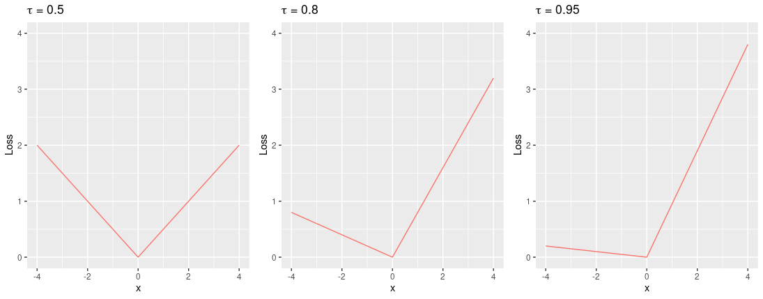
is known as the pinball loss (Koenker, 2005).

Pinball loss for quantiles 0.5, 0.8, 0.95.

We can approximate the above expression empirically given a sample of size $n$ , which gives the quantile estimator, $\hat{\mu}_\tau(\boldsymbol{x}) = \boldsymbol{x}^\mathsf{T} \hat{\boldsymbol{\beta}}$ where

$\hat{\boldsymbol{\beta}} = \underset{\boldsymbol{\beta}}{\arg \min} \frac{1}{n} \sum_{i=1}^n \rho_\tau \left\{y_i - \boldsymbol{x}_i^\mathsf{T} \boldsymbol{\beta}\right\},$

where $\boldsymbol{x}_i$ is the $i$ th vector of covariates, and $\boldsymbol{\beta}$ is vector of regression coefficients.

So far we have described QR, so to turn this into a QGAM we assume $\mu_\tau(\boldsymbol{x})$ has additive structure, that is, we can write the $\tau$ th conditional quantile as

$\mu_\tau(\boldsymbol{x}) = \sum_{j=1}^m f_j(\boldsymbol{x}),$

where the $m$ additive terms are defined in terms of basis functions (e.g. spline bases). A marginal smooth effect could be, for example

$f_j(\boldsymbol{x}) = \sum_{k=1}^{r_j} \beta_{jk} b_{jk}(x_j),$

where $\beta_{jk}$ are unknown coefficients, $b_{jk}(x_j)$ are known spline basis functions and $r_j$ is the basis dimension.

Denote $\boldsymbol{\mathrm{x}}_i$ the vector of basis functions evaluated at $\boldsymbol{x}_i$ , then the $n \times d$ design matrix $\boldsymbol{\mathrm{X}}$ is defined as having $i$ th row $\boldsymbol{\mathrm{x}}_i$ , for $i = 1, \dots, n$ , and $d = r_1+\dots +r_m$ is the total basis dimension over all $f_j$ . Now the quantile estimate is defined as $\mu_\tau(\boldsymbol{x}_i) = \boldsymbol{\mathrm{x}}_i^\mathsf{T} \boldsymbol{\beta}$ . When estimating the regression coefficients, we put a ridge penalty on $\boldsymbol{\beta}_{j}$ to control complexity of $f_j$ , thus we seek to minimise the penalised pinball loss

$V(\boldsymbol{\beta},\boldsymbol{\gamma},\sigma) = \sum_{i=1}^n \frac{1}{\sigma} \rho_\tau \left\{y_i - \mu(\boldsymbol{x}_i)\right\} + \frac{1}{2} \sum_{j=1}^m \gamma_j \boldsymbol{\beta}^\mathsf{T} \boldsymbol{\mathrm{S}}_j \boldsymbol{\beta},$

where $\boldsymbol{\gamma} = (\gamma_1,\dots,\gamma_m)$ is a vector of positive smoothing parameters, $1/\sigma>0$ is the learning rate and the $\boldsymbol{\mathrm{S}}_j$ ‘s are positive semi-definite matrices which penalise the wiggliness of the corresponding effect $f_j$ . Minimising $V$ with respect to $\boldsymbol{\beta}$ given fixed $\sigma$ and $\boldsymbol{\gamma}$ leads to the maximum a posteriori (MAP) estimator $\hat{\boldsymbol{\beta}}$ .

There are a number of methods to tune the smoothing parameters and learning rate. The framework from Fasiolo et al. (2021) consists in:

calibrating $\sigma$ by Integrated Kullback–Leibler minimisation
selecting $\boldsymbol{\gamma}|\sigma$ by Laplace Approximate Marginal Loss minimisation
estimating $\boldsymbol{\beta}|\boldsymbol{\gamma},\sigma$ by minimising penalised Extended Log-F loss (note that this loss is simply a smoothed version of the pinball loss introduced above)

For more detail on what each of these steps means I refer the reader to Fasiolo et al. (2021). Clearly this three-layered nested optimisation can take a long time to converge, especially in cases where we have large datasets which is often the case for energy demand forecasting. So my project approach is to adapt this framework in order to make it less computationally expensive.

Application to Swiss Extreme Rainfall

Here I will briefly discuss one potential application of QGAMs, where we analyse a dataset consisting of observations of the most extreme 12 hourly total rainfall each year for 65 Swiss weather stations between 1981-2015. This data set can be found in the R package gamair and for model fitting I used the package mgcViz.

A basic QGAM for the 50% quantile (i.e. $\tau = 0.5$ ) can be fitted using the following formula

$\mu_i = \beta + \psi(\mathrm{reg}_i) + f_1(\mathrm{nao}_i) + f_2(\mathrm{el}_i) + f_3(\mathrm{Y}_i) + f_4(\mathrm{E}_i,\mathrm{N}_i),$

where $\beta$ is the intercept term, $\psi(\mathrm{reg}_i)$ is a parametric factor for climate region, $f_1, \dots, f_4$ are smooth effects, $\mathrm{nao}_i$ is the Annual North Atlantic Oscillation index, $\mathrm{el}_i$ is the metres above sea level, $\mathrm{Y}_i$ is the year of observation, and $\mathrm{E}_i$ and $\mathrm{N}_i$ are the degrees east and north respectively.

After fitting in mgcViz, we can plot the smooth effects and see how these affect the extreme yearly rainfall in Switzerland.

Fitted smooth effects for North Atlantic Oscillation index, elevation, degrees east and north and year of observation.

From the plots observe the following; as we increase the NAO index we observe a somewhat oscillatory effect on extreme rainfall; when increasing elevation we see a steady increase in extreme rainfall before a sharp drop after an elevation of around 2500 metres; as years increase we see a relatively flat effect on extreme rainfall indicating the extreme rainfall patterns might not change much over time (hopefully the reader won’t regard this as evidence against climate change); and from the spatial plot we see that the south-east of Switzerland appears to be more prone to more heavy extreme rainfall.

We could also look into fitting a 3D spatio-temporal tensor product effect, using the following formula

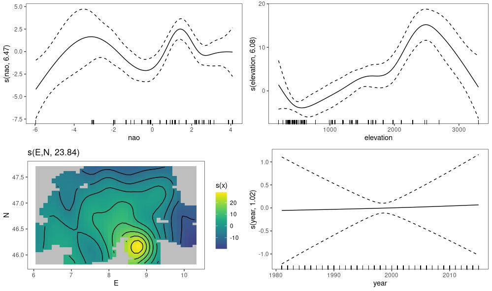
$\mu_i = \beta + \psi(\mathrm{reg}_i) + f_1(\mathrm{nao}_i) + f_2(\mathrm{el}_i) + t(\mathrm{E}_i,\mathrm{N}_i,\mathrm{Y}_i),$

where $t$ is the tensor product effect between $\mathrm{E}_i$ , $\mathrm{N}_i$ and $\mathrm{Y}_i$ . We can examine the spatial effect on extreme rainfall over time by plotting the smooths.

3D spatio-temporal tensor smooths for years 1985, 1995, 2005 and 2015.

There does not seem to be a significant interaction between the location and year, since we see little change between the plots, except for perhaps a slight decrease in the south-east.

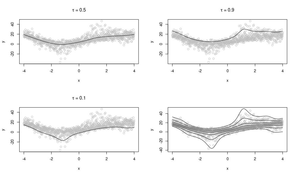
Finally, we can make the most of the QGAM framework by fitting multiple quantiles at once. Here we fit the first formula for quantiles $\tau = 0.1, 0.2, \dots, 0.9$ , and we can examine the fitted smooths for each quantile on the spatial effect.

Spatial smooths for quantiles 0.1, 0.2, …, 0.9.

Interestingly the spatial effect is much stronger in higher quantiles than in the lower ones, where we see a relatively weak effect at the 0.1 quantile, and a very strong effect at the 0.9 quantile ranging between around -30 and +60.

The example discussed here is but one of many potential applications of QGAMs. As mentioned in the introduction, my research area is motivated by energy demand forecasting. My current/future research is focused on adapting the QGAM fitting framework to obtain faster fitting.

References

Fasiolo, M., S. N. Wood, M. Zaffran, R. Nedellec, and Y. Goude (2021). Fast calibrated additive quantile regression. Journal of the American Statistical Association 116 (535), 1402–1412.

Koenker, R. (2005). Quantile Regression. Cambridge University Press.

Student perspectives: Neural Point Processes for Statistical Seismology

Posted on 20th June 202210th August 2022 by sam.stockman

A post by Sam Stockman, PhD student on the Compass programme.

Introduction

Throughout my PhD I aim to bridge a gap between advances made in the machine learning community and the age-old problem of earthquake forecasting. In this cross-disciplinary work with Max Werner from the School of Earth Sciences and Dan Lawson from the School of Mathematics, I hope to create more powerful, efficient and robust models for forecasting, that can make earthquake prone areas safer for their inhabitants.

For years seismologists have sought to model the structure and dynamics of the earth in order to make predictions about earthquakes. They have mapped out the structure of fault lines and conducted experiments in the lab where they submit rock to great amounts of force in order to simulate plate tectonics on a small scale. Yet when trying to forecast earthquakes on a short time scale (that’s hours and days, not tens of years), these models based on the knowledge of the underlying physics are regularly outperformed by models that are statistically motivated. In statistical seismology we seek to make predictions through looking at distributions of the times, locations and magnitudes of earthquakes and use them to forecast the future.

References

[1] – Sofia Dias, Anthony E Ades, Nicky J Welton, Jeroen P Jansen, and Alexander J Sutton. Network meta-analysis for decision-making. John Wiley & Sons, 2018.
[2] – Song F, Altman DG, Glenny AM, Deeks JJ. Validity of indirect comparison for estimating efficacy of competing interventions: empirical evidence from published meta-analyses. Bmj. 2003 Mar 1;326(7387):472.
[3] – David M Phillippo, Anthony E Ades, Sofia Dias, Stephen Palmer, Keith R Abrams, and Nicky J Welton. Methods for population-adjusted indirect comparisons in health technology appraisal. Medical decision making, 38(2):200–211, 2018
[4] – Sofia Dias, Alex J Sutton, AE Ades, and Nicky J Welton. Evidence synthesis for decision making 2: a generalized linear modeling framework for pairwise and network meta-analysis of randomized controlled trials. Medical Decision Making, 33(5):607–617, 2013
[5] – David M Phillippo, Sofia Dias, AE Ades, Mark Belger, Alan Brnabic, Alexander Schacht, Daniel Saure, Zbigniew Kadziola, and Nicky J Welton. Multilevel network meta-regression for population- adjusted treatment comparisons. Journal of the Royal Statistical Society. Series A,(Statistics in Society), 183(3):1189, 2020
[6] – John W Stevens, Christine Fletcher, Gerald Downey, and Anthea Sutton. A review of methods for comparing treatments evaluated in studies that form disconnected networks of evidence. Research synthesis methods, 9(2):148–162, 2018
[7] – Signorovitch, James E., et al. “Matching-adjusted indirect comparisons: a new tool for timely comparative effectiveness research.” Value in Health 15.6 (2012): 940-947.
[8] – Caro JJ, Ishak KJ. No head-to-head trial? Simulate the missing arms. Pharmacoeconomics. 2010;28(10):957–67.
[9] – David M Phillippo, Sofia Dias, AE Ades, Mark Belger, Alan Brnabic, Daniel Saure, Yves Schy-mura, and Nicky J Welton. Validating the assumptions of population adjustment: application of multilevel network meta-regression to a network of treatments for plaque psoriasis. Medical Decision Making, 43(1):53–67, 2023
[10] – Leahy, Joy, et al. “Incorporating single‐arm evidence into a network meta‐analysis using aggregate level matching: assessing the impact.” Statistics in medicine 38.14 (2019): 2505-2523.
") be the conditional c.d.f. of a response,
be the conditional c.d.f. of a response,  , given a
-dimensional vector of covariates,
. In QR we model the
th quantile, that is,
= \inf \{y : F(y|\boldsymbol{x}) \geq \tau\}") .
.
and only need one particular quantile of interest (for example urban planners might only be interested in estimates of extreme rainfall e.g.
). It also allows us to make no assumptions about the underlying true distribution, instead we can model the distribution empirically using multiple quantiles.
= \mathbb{E} \left\{\rho_\tau (y - \mu)| \boldsymbol{x} \right \} = \int \rho_\tau(y - \mu) d F(y|\boldsymbol{x}),")
") , where
, where = (\tau - 1) z \boldsymbol{1}(z<0) + \tau z \boldsymbol{1}(z \geq 0),")
, which gives the quantile estimator,
= \boldsymbol{x}^\mathsf{T} \hat{\boldsymbol{\beta}}") where
where
is the
th vector of covariates, and
is vector of regression coefficients.
") has additive structure, that is, we can write the
has additive structure, that is, we can write the  = \sum_{j=1}^m f_j(\boldsymbol{x}),")
additive terms are defined in terms of basis functions (e.g. spline bases). A marginal smooth effect could be, for example
= \sum_{k=1}^{r_j} \beta_{jk} b_{jk}(x_j),")
are unknown coefficients,
") are known spline basis functions and
are known spline basis functions and  is the basis dimension.
the vector of basis functions evaluated at
design matrix
is defined as having
, and
, and  is the total basis dimension over all
. Now the quantile estimate is defined as
= \boldsymbol{\mathrm{x}}_i^\mathsf{T} \boldsymbol{\beta}") . When estimating the regression coefficients, we put a ridge penalty on
. When estimating the regression coefficients, we put a ridge penalty on  to control complexity of
= \sum_{i=1}^n \frac{1}{\sigma} \rho_\tau \left\{y_i - \mu(\boldsymbol{x}_i)\right\} + \frac{1}{2} \sum_{j=1}^m \gamma_j \boldsymbol{\beta}^\mathsf{T} \boldsymbol{\mathrm{S}}_j \boldsymbol{\beta},")
") is a vector of positive smoothing parameters,
is a vector of positive smoothing parameters,  is the learning rate and the
‘s are positive semi-definite matrices which penalise the wiggliness of the corresponding effect
with respect to
and
and  leads to the maximum a posteriori (MAP) estimator
. by Laplace Approximate Marginal Loss minimisation
by minimising penalised Extended Log-F loss (note that this loss is simply a smoothed version of the pinball loss introduced above)
) can be fitted using the following formula
+ f_1(\mathrm{nao}_i) + f_2(\mathrm{el}_i) + f_3(\mathrm{Y}_i) + f_4(\mathrm{E}_i,\mathrm{N}_i),")
is the intercept term,
") is a parametric factor for climate region,
is a parametric factor for climate region,  are smooth effects,
is the Annual North Atlantic Oscillation index,
is the metres above sea level,
is the year of observation, and
and  are the degrees east and north respectively.
+ f_1(\mathrm{nao}_i) + f_2(\mathrm{el}_i) + t(\mathrm{E}_i,\mathrm{N}_i,\mathrm{Y}_i),")
is the tensor product effect between
, and we can examine the fitted smooths for each quantile on the spatial effect.