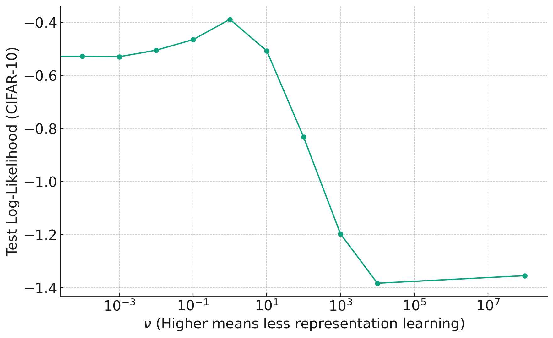
Ed and Ben: In this paper we explore the importance of representation learning in convolutional neural networks, specifically in the context of an infinite-width limit called the Neural Network Gaussian Process (NNGP) that is often used by theorists. Representation learning refers to the ability of models to learn a transformation of the data that is tailored to the task at hand. This is in contrast to algorithms that use a fixed transformation of the data, e.g. a support vector machine with a fixed kernel function like the RBF kernel. Representation learning is thought to be critical to the success of convolutional neural networks in vision tasks, but networks in the NNGP limit do not perform representation learning, instead transforming the data with a fixed kernel function. A recent modification to the NNGP limit, called the Deep Kernel Machine (DKM), allows one to gradually “add representation learning back in” to the NNGP, using a single hyperparameter that controls the amount of flexibility in the kernel. We extend this algorithm to convolutional architectures, which required us to develop a new sparse inducing point approximation scheme. This allowed us to test on the full CIFAR-10 image classification dataset, where we achieved state-of-the-art test accuracy for kernel methods, with 92.7%.
In the plot below, we see how changing the hyperparameter (x-axis) to reduce flexibility too much harms the performance on unseen data.
A post by Codie Wood, PhD student on the Compass programme.
This blog post is an introduction to structure preserving estimation (SPREE) methods. These methods form the foundation of my current work with the Office for National Statistics (ONS), where I am undertaking a six-month internship as part of my PhD. During this internship, I am focusing on the use of SPREE to provide small area estimates of population characteristic counts and proportions.
Small area estimation
Small area estimation (SAE) refers to the collection of methods used to produce accurate and precise population characteristic estimates for small population domains. Examples of domains may include low-level geographical areas, or population subgroups. An example of an SAE problem would be estimating the national population breakdown in small geographical areas by ethnic group [2015_Luna].
Demographic surveys with a large enough scale to provide high-quality direct estimates at a fine-grain level are often expensive to conduct, and so smaller sample surveys are often conducted instead.
SAE methods work by drawing information from different data sources and similar population domains in order to obtain accurate and precise model-based estimates where sample counts are too small for high quality direct estimates. We use the term small area to refer to domains where we have little or no data available in our sample survey.
SAE methods are frequently relied upon for population characteristic estimation, particularly as there is an increasing demand for information about local populations in order to ensure correct allocation of resources and services across the nation.
Structure preserving estimation
Structure preserving estimation (SPREE) is one of the tools used within SAE to provide population composition estimates. We use the term composition here to refer to a population break down into a two-way contingency table containing positive count values. Here, we focus on the case where we have a population broken down into geographical areas (e.g. local authority) and some subgroup or category (e.g. ethnic group or age).
Orginal SPREE-type estimators, as proposed in [1980_Purcell], can be used in the case when we have a proxy data source for our target composition, containing information for the same set of areas and categories but that may not entirely accurately represent the variable of interest. This is usually because the data are outdated or have a slightly different variable definition than the target.
We also incorporate benchmark estimates of the row and column totals for our composition of interest, taken from trusted, quality assured data sources and treated as known values. This ensures consistency with higher level known population estimates. SPREE then adjusts the proxy data to the estimates of the row and column totals to obtain the improved estimate of the target composition.
An illustration of the data required to produce SPREE-type estimates.
In an extension of SPREE, known as generalised SPREE (GSPREE) [2004_Zhang], the proxy data can also be supplemented by sample survey data to generate estimates that are less subject to bias and uncertainty than it would be possible to generate from each source individually. The survey data used is assumed to be a valid measure of the target variable (i.e. it has the same definition and is not out of date), but due to small sample sizes may have a degree of uncertainty or bias for some cells.
The GSPREE method establishes a relationship between the proxy data and the survey data, with this relationship being used to adjust the proxy compositions towards the survey data.
An illustration of the data required to produce GSPREE estimates.
GSPREE is not the only extension to SPREE-type methods, but those are beyond the scope of this post. Further extensions such as Multivariate SPREE are discussed in detail in [2016_Luna].
Original SPREE methods
First, we describe original SPREE-type estimators. For these estimators, we require only well-established estimates of the margins of our target composition.
We will denote the target composition of interest by $\mathbf{Y} = (Y{aj})$, where $Y{aj}$ is the cell count for small area $a = 1,\dots,A$ and group $j = 1,\dots,J$. We can write $\mathbf Y$ in the form of a saturated log-linear model as the sum of four terms,
There are multiple ways to write this parameterisation, and here we use the centered constraints parameterisation given by $$\alpha_0^Y = \frac{1}{AJ}\sum_a\sum_j\log Y_{aj},$$ $$\alpha_a^Y = \frac{1}{J}\sum_j\log Y_{aj} – \alpha_0^Y,$$ $$\alpha_j^Y = \frac{1}{A}\sum_a\log Y_{aj} – \alpha_0^Y,$$ $$\alpha_{aj}^Y = \log Y_{aj} – \alpha_0^Y – \alpha_a^Y – \alpha_j^Y,$$
which satisfy the constraints $\sum_a \alpha_a^Y = \sum_j \alpha_j^Y = \sum_a \alpha_{aj}^Y = \sum_j \alpha_{aj}^Y = 0.$
Using this expression, we can decompose $\mathbf Y$ into two structures:
The association structure, consisting of the set of $AJ$ interaction terms $\alpha_{aj}^Y$ for $a = 1,\dots,A$ and $j = 1,\dots,J$. This determines the relationship between the rows (areas) and columns (groups).
The allocation structure, consisting of the sets of terms $\alpha_0^Y, \alpha_a^Y,$ and $\alpha_j^Y$ for $a = 1,\dots,A$ and $j = 1,\dots,J$. This determines the size of the composition, and differences between the sets of rows (areas) and columns (groups).
Suppose we have a proxy composition $\mathbf X$ of the same dimensions as $\mathbf Y$, and we have the sets of row and column margins of $\mathbf Y$ denoted by $\mathbf Y_{a+} = (Y_{1+}, \dots, Y_{A+})$ and $\mathbf Y_{+j} = (Y_{+1}, \dots, Y_{+J})$, where $+$ substitutes the index being summed over.
We can then use iterative proportional fitting (IPF) to produce an estimate $\widehat{\mathbf Y}$ of $\mathbf Y$ that preserves the association structure observed in the proxy composition $\mathbf X$. The IPF procedure is as follows:
Rescale the rows of $\mathbf X$ as $$ \widehat{Y}_{aj}^{(1)} = X_{aj} \frac{Y_{+j}}{X_{+j}},$$
Rescale the columns of $\widehat{\mathbf Y}^{(1)}$ as $$ \widehat{Y}_{aj}^{(2)} = \widehat{Y}_{aj}^{(1)} \frac{Y_{a+}}{\widehat{Y}_{a+}^{(1)}},$$
Rescale the rows of $\widehat{\mathbf Y}^{(2)}$ as $$ \widehat{Y}_{aj}^{(3)} = \widehat{Y}_{aj}^{(2)} \frac{Y_{+j}}{\widehat{Y}_{+j}^{(2)}}.$$
Steps 2 and 3 are then repeated until convergence occurs, and we have a final composition estimate denoted by $\widehat{\mathbf Y}^S$ which has the same association structure as our proxy composition, i.e. we have $\alpha_{aj}^X = \alpha_{aj}^Y$ for all $a \in \{1,\dots,A\}$ and $j \in \{1,\dots,J\}.$ This is a key assumption of the SPREE implementation, which in practise is often restrictive, motivating a generalisation of the method.
Generalised SPREE methods
If we can no longer assume that the proxy composition and target compositions have the same association structure, we instead use the GSPREE method first introduced in [2004_Zhang], and incorporate survey data into our estimation process.
The GSPREE method relaxes the assumption that $\alpha_{aj}^X = \alpha_{aj}^Y$ for all $a \in \{1,\dots,A\}$ and $j \in \{1,\dots,J\},$ instead imposing the structural assumption $\alpha_{aj}^Y = \beta \alpha_{aj}^X$, i.e. the association structure of the proxy and target compositions are proportional to one another. As such, we note that SPREE is a particular case of GSPREE where $\beta = 1$.
Continuing with our notation from the previous section, we proceed to estimate $\beta$ by modelling the relationship between our target and proxy compositions as a generalised linear structural model (GLSM) given by
$$\tau_{aj}^Y = \lambda_j + \beta \tau_{aj}^X,$$ with $\sum_j \lambda_j = 0$, and where $$ \begin{align} \tau_{aj}^Y &= \log Y_{aj} – \frac{1}{J}\sum_j\log Y_{aj},\\
&= \alpha_{aj}^Y + \alpha_j^Y,
\end{align}$$ and analogously for $\mathbf X$.
It is shown in [2016_Luna] that fitting this model is equivalent to fitting a Poisson generalised linear model to our cell counts, with a $\log$ link function. We use the association structure of our proxy data, as well as categorical variables representing the area and group of the cell, as our covariates. Then we have a model given by $$\log Y_{aj} = \gamma_a + \tilde{\lambda}_j + \tilde{\beta}\alpha_{aj}^X,$$ with $\gamma_a = \alpha_0^Y + \alpha_a^Y$, $\tilde\lambda_j = \alpha_j^Y$ and $\tilde\beta \alpha_{aj}^X = \alpha_{aj}^Y.$
When fitting the model we use survey data $\tilde{\mathbf Y}$ as our response variable, and are then able to obtain a set of unbenchmarked estimates of our target composition. The GSPREE method then benchmarks these to estimates of the row and column totals, following a procedure analagous to that undertaken in the orginal SPREE methodology, to provide a final set of estimates for our target composition.
ONS applications
The ONS has used GSPREE to provide population ethnicity composition estimates in intercensal years, where the detailed population estimates resulting from the census are outdated [2015_Luna]. In this case, the census data is considered the proxy data source. More recent works have also used GSPREE to estimate counts of households and dwellings in each tenure at the subnational level during intercensal years [2023_ONS].
My work with the ONS has focussed on extending the current workflows and systems in place to implement these methods in a reproducible manner, allowing them to be applied to a wider variety of scenarios with differing data availability.
References
[1980_Purcell] Purcell, Noel J., and Leslie Kish. 1980. ‘Postcensal Estimates for Local Areas (Or Domains)’. International Statistical Review / Revue Internationale de Statistique 48 (1): 3–18. https://doi.org/10/b96g3g.
[2004_Zhang] Zhang, Li-Chun, and Raymond L. Chambers. 2004. ‘Small Area Estimates for Cross-Classifications’. Journal of the Royal Statistical Society Series B: Statistical Methodology 66 (2): 479–96. https://doi.org/10/fq2ftt.
[2015_Luna] Luna Hernández, Ángela, Li-Chun Zhang, Alison Whitworth, and Kirsten Piller. 2015. ‘Small Area Estimates of the Population Distribution by Ethnic Group in England: A Proposal Using Structure Preserving Estimators’. Statistics in Transition New Series and Survey Methodology 16 (December). https://doi.org/10/gs49kq.
[2016_Luna] Luna Hernández, Ángela. 2016. ‘Multivariate Structure Preserving Estimation for Population Compositions’. PhD thesis, University of Southampton, School of Social Sciences. https://eprints.soton.ac.uk/404689/.
A post by Ben Anson, PhD student on the Compass programme.
Semantic Search
Semantic search is here. We already see it in use in search engines [13], but what is it exactly and how does it work?
Search is about retrieving information from a corpus, based on some query. You are probably using search technology all the time, maybe $\verb|ctrl+f|$, or searching on google. Historically, keyword search, which works by comparing the occurrences of keywords between queries and documents in the corpus, has been surprisingly effective. Unfortunately, keywords are inherently restrictive – if you don’t know the right one to use then you are stuck.
Semantic search is about giving search a different interface. Semantic search queries are provided in the most natural interface for humans: natural language. A semantic search algorithm will ideally be able to point you to a relevant result, even if you only provided the gist of your desires, and even if you didn’t provide relevant keywords.
Figure 1: Illustration of semantic search and keyword search models
Figure 1 illustrates a concrete example where semantic search might be desirable. The query ‘animal’ should return both the dog and cat documents, but because the keyword ‘animal’ is not present in the cat document, the keyword model fails. In other words, keyword search is susceptible to false negatives.
Transformer neural networks turn out to be very effective for semantic search [1,2,3,10]. In this blog post, I hope to elucidate how transformers are tuned for semantic search, and will briefly touch on extensions and scaling.
The search problem, more formally
Suppose we have a big corpus $\mathcal{D}$ of documents (e.g. every document on wikipedia). A user sends us a query $q$, and we want to point them to the most relevant document $d^*$. If we denote the relevance of a document $d$ to $q$ as $\text{score}(q, d)$, the top search result should simply be the document with the highest score,
This framework is simple and it generalizes. For $\verb|ctrl+f|$, let $\mathcal{D}$ be the set of individual words in a file, and $\text{score}(q, d) = 1$ if $q=d$ and $0$ otherwise. The venerable keyword search algorithm BM25 [4], which was state of the art for decades [8], uses this score function.
For semantic search, the score function is often set as the inner product between query and document embeddings: $\text{score}(q, d) = \langle \phi(q), \phi(d) \rangle$. Assuming this score function actually works well for finding relevant documents, and we use a simple inner product, it is clear that the secret sauce lies in the embedding function $\phi$.
Transformer embeddings
We said above that a common score function for semantic search is $\text{score}(q, d) = \langle \phi(q), \phi(d) \rangle$. This raises two questions:
Question 1: what should the inner product be? For semantic search, people tend to use the cosine similarity for their inner product.
Question 2: what should $\phi$ be? The secret sauce is to use a transformer encoder, which is explained below.
Quick version
Transformers magically gives us a tunable embedding function $\phi: \text{“set of all pieces of text”} \rightarrow \mathbb{R}^{d_{\text{model}}}$, where $d_{\text{model}}$ is the embedding dimension.
More detailed version
See Figure 2 for an illustration of how a transformer encoder calculates an embedding for a piece of text. In the figure we show how to encode “cat”, but we can encode arbitrary pieces of text in a similar way. The transformer block details are out of scope here; though, for these details I personally found Attention is All You Need [9] helpful, the crucial part being the Multi-Head Attention which allows modelling dependencies between words.
Figure 2: Transformer illustration (transformer block image taken from [6])
The transformer encoder is very flexible, with almost every component parameterized by a learnable weight / bias – this is why it can be used to model the complicated semantics in natural language. The pooling step in Figure 2, where we map our sequence embedding $X’$ to a fixed size, is not part of a ‘regular’ transformer, but it is essential for us. It ensures that our score function $\langle \phi(q), \phi(d) \rangle$ will work when $q$ and $d$ have different sizes.
Making the score function good for search
There is a massive issue with transformer embedding as described above, at least for our purposes – there is no reason to believe it will satisfy simple semantic properties, such as,
$\text{score}(\text{“busy place”}, \text{“tokyo”}) > \text{score}(\text{“busy place”}, \text{“a small village”})$
‘But why would the above not work?’ Because, of course, transformers are typically trained to predict the next token in a sequence, not to differentiate pieces of text according to their semantics.
The solution to this problem is not to eschew transformer embeddings, but rather to fine-tune them for search. The idea is to encourage the transformer to give us embeddings that place semantically dissimilar items far apart. E.g. let $q=$’busy place’, then we want $ d^+=$’tokyo’ to be close to $q$ and $d^-=$’a small village’ to be far away.
This semantic separation can be achieved by fine-tuning with a contrastive loss [1,2,3,10],
where $\theta$ represents the transformer parameters. The $\exp$’s in the contastive loss are to ensure we never divide by zero. Note that we can interpret the contrastive loss as doing classification since we can think of the argument to the logarithm as $p(d^+ | q)$.
That’s all we need, in principle, to turn a transformer encoder into a text embedder! In practice, the contrastive loss can be generalized to include more positive and negative examples, and it is indeed a good idea to have a large batch size [11] (intuitively it makes the separation of positive and negative examples more difficult, resulting in a better classifier). We also need a fine-tuning dataset – a dataset of positive/negative examples. OpenAI showed that it is possible to construct one in an unsupervised fashion [1]. However, there are also publicly available datasets for supervised fine-tuning, e.g. MSMARCO [12].
Extensions
One really interesting avenue of research is training of general purposes encoders. The idea is to provide instructions alongside the queries/documents [2,3]. The instruction could be $\verb|Embed this document for search: {document}|$ (for the application we’ve been discussing), or $\verb|Embed this document for clustering: {document}|$ to get embeddings suitable for clustering, or $\verb|Embed this document for sentiment analysis: {document}|$ for embeddings suitable for sentiment analysis. The system is fine-tuned end-to-end with the appropriate task, e.g. a contrastive learning objective for the search instruction, a classification objective for sentiment analysis, etc., leaving us with an easy way to generate embeddings for different tasks.
A note on scaling
The real power of semantic (and keyword) search comes when a search corpus is too large for a human to search manually. However if the corpus is enormous, we’d rather avoid looking at every document each time we get a query. Thankfully, there are methods to avoid this by using specially tailored data structures: see Inverted Indices for keyword algorithms, and Hierarchical Navigable Small World graphs [5] for semantic algorithms. These both reduce search time complexity from $\mathcal{O}(|\mathcal{D}|)$ to $\mathcal{O}(\log |\mathcal{D}|)$, where $|\mathcal{D}|$ is the corpus size.
There are many startups (Pinecone, Weviate, Milvus, Chroma, etc.) that are proposing so-called vector databases – databases in which embeddings are stored, and queries can be efficiently performed. Though, there is also work contesting the need for these types of database in the first place [7].
Summary
We summarised search, semantic search, and how transformers are fine-tuned for search with a contrastive loss. I personally find this a very nice area of research with exciting real-world applications – please reach out (ben.anson@bristol.ac.uk) if you’d like to discuss it!
References
[1]: Text and code embeddings by contrastive pre-training, Neelakantan et al (2022)
[2]: Task-aware Retrieval with Instructions, Asai et al (2022)
[3]: One embedder, any task: Instruction-finetuned text embeddings, Su et al (2022)
[4]: Some simple effective approximations to the 2-poisson model for probabilistic weighted retrieval, Robertson and Walker (1994)
[5]: Efficient and robust approximate nearest neighbor search using Hierarchical Navigable Small World graphs, https://arxiv.org/abs/1603.09320
[6]: An Image is Worth 16×16 Words: Transformers for Image Recognition at Scale, https://arxiv.org/abs/2010.11929
[7]: Vector Search with OpenAI Embeddings: Lucene Is All You Need, arXiv preprint arXiv:2308.14963
[8]: Complement lexical retrieval model with semantic residual embeddings, Advances in Information Retrieval (2021)
[9]: Attention is all you need, Advances in neural information processing systems (2017)
A post by Josh Givens, PhD student on the Compass programme.
Density ratio estimation is a highly useful field of mathematics with many applications. This post describes my research undertaken alongside my supervisors Song Liu and Henry Reeve which aims to make density ratio estimation robust to missing data. This work was recently published in proceedings for AISTATS 2023.
Density Ratio Estimation
Definition
As the name suggests, density ratio estimation is simply the task of estimating the ratio between two probability densities. More precisely for two RVs (Random Variables) on some space with probability density functions (PDFs) respectively, the density ratio is the function defined by
.
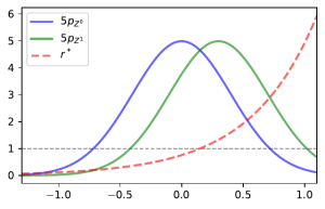
Plot of the scaled density ratio alongside the PDFs for the two classes.
Density ratio estimation (DRE) is then the practice of using IID (independent and identically distributed) samples from and to estimate . What makes DRE so useful is that it gives us a way to characterise the difference between these 2 classes of data using just 1 quantity, .
The Density Ratio in Classification
We now give demonstrate this characterisability in the case of classification. To frame this as a classification problem define and by . The task of predicting given using some function is then our standard classification problem. In classification a common target is the Bayes Optimal Classifier, the classifier which maximises We can write this classifier in terms of as we know that where is the indicator function. Then, by the total law of probability, we have
Hence to learn the Bayes optimal classifier it is sufficient to learn the density ratio and a constant. This pattern extends well beyond Bayes optimal classification to many other areas such as error controlled classification, GANs, importance sampling, covariate shift, and others. Generally speaking, if you are in any situation where you need to characterise the difference between two classes of data, it’s likely that the density ratio will make an appearance.
Estimation Implementation – KLIEP
Now we have properly introduced and motivated DRE, we need to look at how we can go about performing it. We will focus on one popular method called KLIEP here but there are a many different methods out there (see Sugiyama et al 2012 for some additional examples.)
The intuition behind KLIEP is simple: as , if is “close” to then is a good estimate of . To measure this notion of closeness KLIEP uses the KL (Kullback-Liebler) divergence which measures the distance between 2 probability distributions. We can now formulate our ideal KLIEP objective as follows:
where represent the KL divergence from to . The constraint ensures that the right hand side of our KL divergence is indeed a PDF. From the definition of the KL-divergence we can rewrite the solution to this as where is the solution to the unconstrained optimisation
As this is now just an unconstrained optimisation over expectations of known transformations of , we can approximate this using samples. Given samples from and samples from our estimate of the density ratio will be where solves
Despite KLIEP being commonly used, up until now it has not been made robust to missing not at random data. This is what our research aims to do.
Missing Data
Suppose that instead of observing samples from , we observe samples from some corrupted version of , . We assume that so that either is missing or takes the value of . We also assume that whether is missing depends upon the value of . Specifically we assume with not constant and refer to as the missingness function. This type of missingness is known as missing not at random (MNAR) and when dealt with improperly can lead to biased result. Some examples of MNAR data could be readings take from a medical instrument which is more likely to err when attempting to read extreme values or recording responses to a questionnaire where respondents may be more likely to not answer if the deem their response to be unfavourable. Note that while we do not see what the true response would be, we do at least get a response meaning that we know when an observation is missing.
Missing Data with DRE
We now go back to density ratio estimation in the case where instead of observing samples from we observe samples from their corrupted versions . We take their respective missingness functions to be and assume them to be known. Now let us look at what would happen if we implemented KLIEP with the data naively by simply filtering out the missing-values. In this case, the actual density ratio we would be estimating would be
and so we would get inaccurate estimates of the density ratio no matter how many samples are used to estimate it. The image below demonstrates this in the case were samples in class are more likely to be missing when larger and class has no missingness.
A plot of the density ratio using both the full data and only the observed part of the corrupted data
Our Solution
Our solution to this problem is to use importance weighting. Using relationships between the densities of and we have that
As such we can re-write the KLIEP objective to keep our expectation estimation unbiased even when using these corrupted samples. This gives our modified objective which we call M-KLIEP as follows. Given samples from and samples from our estimate is where solves
This objective will now target even when used on MNAR data.
Application to Classification
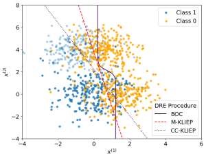
We now apply our density ratio estimation on MNAR data to estimate the Bayes optimal classifier. Below shows a plot of samples alongside the true Bayes optimal classifier and estimated classifiers from the samples via our method M-KLIEP and a naive method CC-KLIEP which simply ignores missing points. Missing data points are faded out.
Faded points represent missing values. M-KLIEP represents our method, CC-KLIEP represents a Naive approach, BOC gives the Bayes optimal classifier
As we can see, due to not accounting for the MNAR nature of the data, CC-KLIEP underestimates the true number of class 1 samples in the top left region and therefore produces a worse classifier than our approach.
Additional Contributions
As well as this modified objective our paper provides the following additional contributions:
Theoretical finite sample bounds on the accuracy of our modified procedure.
Methods for learning the missingness functions .
Expansions to partial missingness via a Naive-Bayes framework.
Downstream implementation of our method within Neyman-Pearson classification.
Adaptations to Neyman-Pearson classification itself making it robust to MNAR data.
Givens, J., Liu, S., & Reeve, H. W. J. (2023). Density ratio estimation and neyman pearson classification with missing data. In F. Ruiz, J. Dy, & J.-W. van de Meent (Eds.), Proceedings of the 26th international conference on artificial intelligence and statistics (Vol. 206, pp. 8645–8681). PMLR.
Sugiyama, M., Suzuki, T., & Kanamori, T. (2012). Density Ratio Estimation in Machine Learning. Cambridge University Press.
Ant Stephenson, Jack Simons, and I (Dan Ward) had the pleasure of attending the 2022 Conference on Neural Information Processing Systems (NeurIPS), one of the largest machine learning conferences in the world. The conference was held in New Orleans, which gave us an opportunity to explore a lively city full of culture with delicious local cuisine. We thought we’d collaborate on a blog post together covering some of the highlights.
Memorable Talks
The conference had broad range of talks including technical presentations of research, applied projects, and discussions of the philosophical and ethical questions that arise in AI. To give a taste of some of the talks, we picked out some of our favourites below.
Noam Brown: Human Modelling and Strategic Reasoning in the Game of Diplomacy.
The Game of Diplomacy is a strategic board game invented in 1954. It’s unique feature, and of crucial importance of the game, is that players interact via natural language to form allegiances. Whilst AI has been successful in beating humans in many purely adversarial games (e.g. Chess, Go), this collaborative element poses unique challenges. Firstly, it isn’t obvious how to evaluate/devise strategies for collaboration/betrayal, especially in the self-play-based reinforcement learning paradigm. Secondly, as communication happens via natural language, the AI must be able to translate their strategic plan into text. This strange combination of problems lead to interesting and innovative solutions. Paper link here.
Geoffrey Hinton: The Forward-Forward Algorithm for Training Deep Neural Networks.
Among the great line-up of speakers was Professor Geoffrey Hinton, known for popularising backpropogation for deep neural networks. Inspired by producing a more biologically plausible algorithm for learning, he has proposed the ‘Forward-Forward’ algorithm which he claims can also explain the phenomena of sleep! Professor Geoffrey Hinton then went on to express his belief that using biologically-inspired hardware, so-called neuromorphic computing, may play a key role in advancing AI. The talk was certainly unconventional, but nevertheless entertaining. Paper link here.
David Chalmers: Could a Large Language Model be Conscious?
Amongst all the machine-learning experts was David Chalmers, a philosopher! There are important questions regarding the possibility that language models might be conscious. David Chalmers aimed to educate the machine-learning audience in attendance of how we can better think about these problems and re-phrase the questions that we’re asking. We concluded that these questions are, unsurprisingly, best left to philosophers!
Poster Sessions
Jack and Dan:
I (Dan), presented a poster of my work at the conference, on Robust Neural Posterior Estimation (paper link here). I was definitely surprised by the scale of the poster sessions, and the broad scope of all the work taking place. Below is some of the posters that me and Jack found interesting:
Contrastive Neural Ratio Estimation Benjamin K. Miller · Christoph Weniger · Patrick Forré Authors propose NRE-C which aims to generalise NRE-A (Hermans et al. (2019)) and NRE-B (Durkan et al. (2020)) into one method. NRE-C can recover both methods by taking their two introduced hyperparameters at certain limits. Paper link here.
Towards Reliable Simulation-Based Inference with Balanced Neural Ratio Estimation Arnaud Delaunoy · Joeri Hermans · François Rozet · Antoine Wehenkel · Gilles Louppe These authors also make a contribution to the field of neural ratio estimation in the simulation-based inference context. Authors propose the notion of a “balanced” classifier, which is a classifier in which the average output from the classifier over the positive data class plus the average output over the negative data class equals to 1. The authors argue that if one has a classifier is balanced then it will lead to more conservative posterior estimates, which is something which practitioners seek. To integrate this into an algorithm they suggest adding a penalisation term onto the standard logistic-loss which punishes classifiers as they become less balanced. Paper link here.
Training and Inference on Any-Order Autoregressive Models the Right Way Andy Shih · Dorsa Sadigh · Stefano Ermon A joint distribution can be decomposed into its univariate conditionals by the chain rule, although by doing so we implicitly choose an ordering in a model, which prevents arbitrary conditional inference. Any-order autoregressive models circumvent this generally by being trained such that all possible univariate conditionals are considered, but this leads to learning redundant information. The paper proposes a new method to train autoregressive models, using a subset of univariate conditionals that still supports arbitrary conditional inference. This research was also presented as a talk, but sadly we missed it! Paper link here.
Anthony:
The poster sessions formed the bulk of the conference timetable, with 2 2-hour sessions per day, on Tuesday, Wednesday and Thursday. These were very busy, with many posters on a wide-range of topics and a large congregation of attendees. As a result, it was sometimes difficult to track down the subset of posters on material of particular interest and when this feat was achieved, on occasion it was still hard work to actually have a detailed conversation with the author(s). Nonetheless, it was interesting to see the how varied the subjects of the poster were and in addition get a feeling for “themes” of the conference: recurring, clearly in-vogue topics. Amongst the sea of posters, I did manage to find a number relating to GPs; of these, those I found most interesting were:
Posterior and Computational Uncertainty in Gaussian Processes: Jonathan Wenger · Geoff Pleiss · Marvin Pförtner · Philipp Hennig · John Cunningham Here the authors propose a way to naturally incorporate uncertainty introduced from the use of (iterative) GP approximation methods. Paper link here.
Sparse Gaussian Process Hyperparameters: Optimize or Integrate? Vidhi Lalchand · Wessel Bruinsma · David Burt · Carl Edward Rasmussen
The authors attempt to integrate a fully-Bayesian inference procedure for sparse GPs, as an alternative to the commonly adopted approach of optimising the kernel hyperparameters by maximum likelihood estimation. Paper link here.
Log-Linear-Time Gaussian Processes Using Binary Tree Kernels: Michael K. Cohen · Samuel Daulton · Michael A Osborne
The idea here feels a bit unorthodox; they use a “binary-tree” kernel which discretises the space, with quantization error determined by the number of leaves. This would seem to lose interpretability on the properties of the function prior (e.g. smoothness), but does appear to give empirical benefits in their experiments. Paper link here.
Workshops
In addition to the main conference, on the Friday and Saturday at the end of the week there were a selection of workshops on a variety of sub-fields within machine learning. If you are fortunate enough for there to be a workshop dedicated to your research area, then they provide a space to gather people with research directly relevant to your own and facilitate helpful discussions and networking opportunities.
Anthony:
For me, the “Gaussian processes, spatiotemporal modeling and decision-making systems” workshop was the most useful part of the conference. It gave me the chance to speak to people working on interesting problems related to my own; discover the kind of directions they are heading in and lines of work they are contemplating. Additionally, I presented a poster during this workshop which allowed me to discuss my work with an audience well-versed on the topic and its possible significance.
The Big Easy
In addition to the actual conference, attending NeurIPS also gave us the opportunity to explore the city of New Orleans; aka The Big Easy. Upon arrival, we were immediately greeted in the airport by the sound of Louis Armstrong, a strong theme in the city, which features a park named after him. New ‘Awlins’ is well known for its jazz, but awareness of this fact does not necessarily prepare you for the sheer quantity, especially in the streets of the French Quarter, that awaits you. The real epicentre of jazz in the city is situated on Frenchmen street, on which a swathe of bars hosting nearly-nightly live music reside. We spent several evenings there, including one of particular note, where French president Emmanuel Macron suddenly appeared, trailed by an extensive retinue of blue-suited aides and bodyguards. Another street in New Orleans infamous for its nightlife is Bourbon street. Where Frenchmen street is focused on jazz, Bourbon street contains all manner of rowdy madness, assaulting your senses with noise, smells and sights as soon as you arrive. Both are necessary experiences when visiting The Big Easy.
Conclusion
All in all, the conference was a great opportunity to get a taste of the massive array of research that occurs in machine learning. We were all surprised by the scope of the research topics and talks, and enjoyed the opportunity to explore a new culture and city.
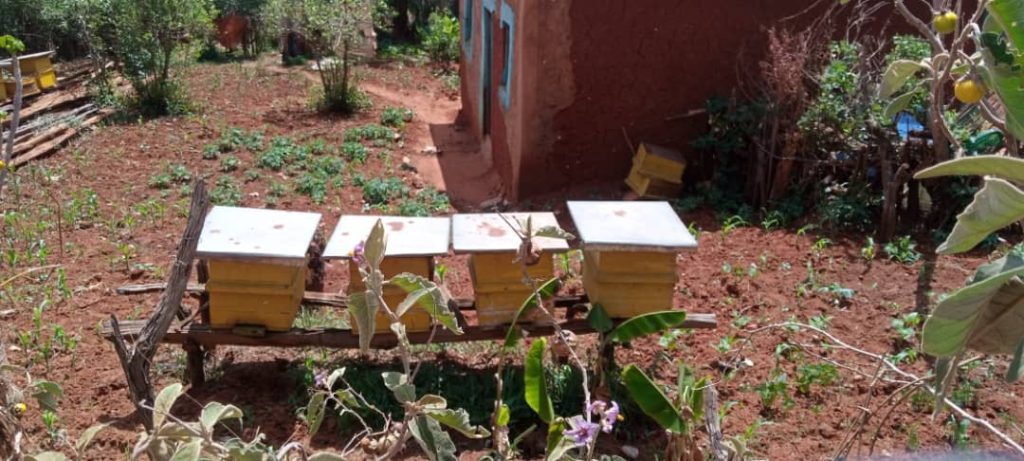
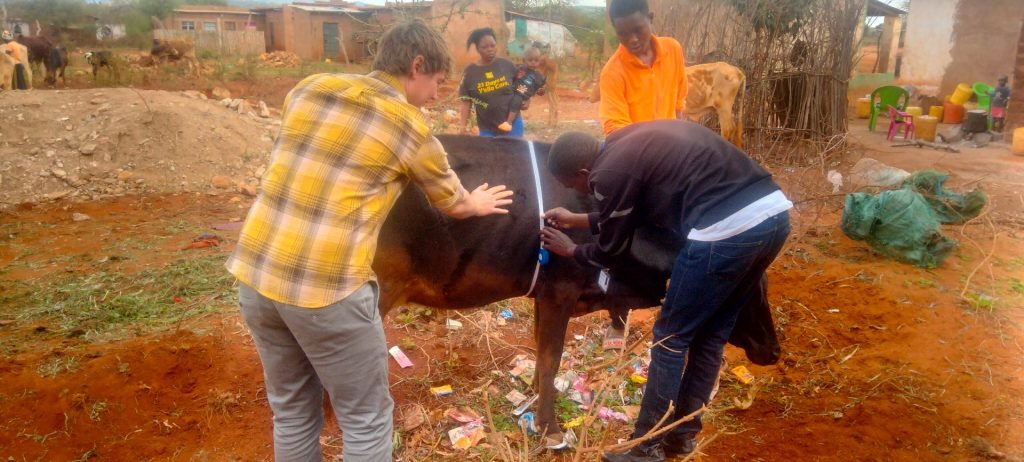
This blog describes an approach being developed to deliver rapid classification of farmer strategies. The data comes from a survey conducted with two groups of smallholder farmers (see image 2), one group living in the Taita Hills area of southern Kenya and the other in Yebelo, southern Ethiopia. This work would not have been possible without the support of my supervisors James Hammond, from the International Livestock Research Institute (ILRI) (and developer of the Rural Household Multi Indicator Survey, RHoMIS, used in this research), as well as Andrew Dowsey, Levi Wolf and Kate Robson Brown from the University of Bristol.
Image 2: Measuring a Cows Heart Girth as Part of the Farm Surveys
Aims of the project
The goal of my PhD is to contribute a landscape approach to analysing agricultural systems. On-farm practices are an important part of an agricultural system and are one of the trilogy of components that make-up what Rizzo et al (2022) call ‘agricultural landscape dynamics’ – the other two components being Natural Resources and Landscape Patterns. To understand how a farm interacts with and responds to Natural Resources and Landscape Patterns it seems sensible to try and understand not just each farms inputs and outputs but its overall strategy and component practices. (more…)


 on some space
  with probability density functions (PDFs)
  respectively, the density ratio is the function
  defined by
:=\frac{p_0(z)}{p_1(z)}") .
.
 and
and  to estimate
  . What makes DRE so useful is that it gives us a way to characterise the difference between these 2 classes of data using just 1 quantity,
 ") and
and  by
by  . The task of predicting
  given
given  is then our standard classification problem. In classification a common target is the Bayes Optimal Classifier, the classifier
  which maximises
 ).") We can write this classifier in terms of
We can write this classifier in terms of =\mathbb{I}\{\mathbb{P}(Y=1|Z=z)>0.5\}") where
where  is the indicator function. Then, by the total law of probability, we have
=\frac{p_{Z|Y=1}(z)\mathbb{P}(Y=1)}{p_{Z|Y=1}(z)\mathbb{P}(Y=1)+p_{Z|Y=0}(z)\mathbb{P}(Y=0)}")
\mathbb{P}(Y=1)}{p_1(z)\mathbb{P}(Y=1)+p_0(z)\mathbb{P}(Y=0)} =\frac{1}{1+\frac{1}{r}\frac{\mathbb{P}(Y=0)}{\mathbb{P}(Y=1)}}.")
 , if
, if  is “close” to
  then
then  is a good estimate of
 ")
p_0(z)\mathrm{d}z=1")
") represent the KL divergence from
represent the KL divergence from  to
to  . The constraint ensures that the right hand side of our KL divergence is indeed a PDF. From the definition of the KL-divergence we can rewrite the solution to this as
 ![\hat r:=\frac{\tilde r}{\mathbb{E}[r(X^0)]}](https://s0.wp.com/latex.php?latex=%5Chat+r%3A%3D%5Cfrac%7B%5Ctilde+r%7D%7B%5Cmathbb%7BE%7D%5Br%28X%5E0%29%5D%7D&bg=ffffff&fg=000000&s=0 "\hat r:=\frac{\tilde r}{\mathbb{E}[r(X^0)]}") where
where  is the solution to the unconstrained optimisation
![\underset{r}{\text{min}}~\mathbb{E}[\log (r(Z^1))]-\log(\mathbb{E}[r(Z^0)]).](https://s0.wp.com/latex.php?latex=%5Cunderset%7Br%7D%7B%5Ctext%7Bmin%7D%7D%7E%5Cmathbb%7BE%7D%5B%5Clog+%28r%28Z%5E1%29%29%5D-%5Clog%28%5Cmathbb%7BE%7D%5Br%28Z%5E0%29%5D%29.&bg=ffffff&fg=000000&s=2 "\underset{r}{\text{min}}~\mathbb{E}[\log (r(Z^1))]-\log(\mathbb{E}[r(Z^0)]).")
 from
from  and samples
  from
from  our estimate of the density ratio will be
 \right)^{-1}\tilde r") where
where )-\log\left(\frac{1}{n}\sum_{i=1}^n r(z^0_i)\right).")
 . We assume that
 =1") so that either
so that either =\varphi(z)") with
with ") not constant and refer to
not constant and refer to  as the missingness function. This type of missingness is known as missing not at random (MNAR) and when dealt with improperly can lead to biased result. Some examples of MNAR data could be readings take from a medical instrument which is more likely to err when attempting to read extreme values or recording responses to a questionnaire where respondents may be more likely to not answer if the deem their response to be unfavourable. Note that while we do not see what the true response would be, we do at least get a response meaning that we know when an observation is missing.
 we observe samples from their corrupted versions
  . We take their respective missingness functions to be
  and assume them to be known. Now let us look at what would happen if we implemented KLIEP with the data naively by simply filtering out the missing-values. In this case, the actual density ratio we would be estimating would be
:=\frac{p_{X_1|X_1\neq\varnothing}(z)}{p_{X_0|X_o\neq\varnothing}(z)}\propto\frac{(1-\varphi_1(z))p_1(z)}{(1-\varphi_0(z))p_0(z)}\not{\propto}r^*(z)")
 are more likely to be missing when larger and class
  has no missingness.
![\mathbb{E}[g(Z)]=\mathbb{E}\left[\frac{\mathbb{I}\{X\neq\varnothing\}g(X)}{1-\varphi(X)}\right].](https://s0.wp.com/latex.php?latex=%5Cmathbb%7BE%7D%5Bg%28Z%29%5D%3D%5Cmathbb%7BE%7D%5Cleft%5B%5Cfrac%7B%5Cmathbb%7BI%7D%5C%7BX%5Cneq%5Cvarnothing%5C%7Dg%28X%29%7D%7B1-%5Cvarphi%28X%29%7D%5Cright%5D.&bg=ffffff&fg=000000&s=2 "\mathbb{E}[g(Z)]=\mathbb{E}\left[\frac{\mathbb{I}\{X\neq\varnothing\}g(X)}{1-\varphi(X)}\right].")
 from
from  and samples
  from
from  our estimate is
 }{1-\varphi_o(x_i^o)}\right)^{-1}\tilde r") where
where )}{1-\varphi_1(x_i^1)}-\log\left(\frac{1}{n}\sum_{i=1}^n\frac{\mathbb{I}\{x_i^0\neq\varnothing\}r(x_i^0)}{1-\varphi_0(x_i^0)}\right).")
 .
.