A post by Ben Anson, PhD student on the Compass programme.
Semantic Search
Semantic search is here. We already see it in use in search engines [13], but what is it exactly and how does it work?
Search is about retrieving information from a corpus, based on some query. You are probably using search technology all the time, maybe $\verb|ctrl+f|$, or searching on google. Historically, keyword search, which works by comparing the occurrences of keywords between queries and documents in the corpus, has been surprisingly effective. Unfortunately, keywords are inherently restrictive – if you don’t know the right one to use then you are stuck.
Semantic search is about giving search a different interface. Semantic search queries are provided in the most natural interface for humans: natural language. A semantic search algorithm will ideally be able to point you to a relevant result, even if you only provided the gist of your desires, and even if you didn’t provide relevant keywords.

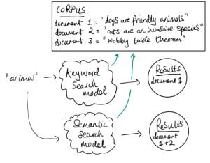
Figure 1 illustrates a concrete example where semantic search might be desirable. The query ‘animal’ should return both the dog and cat documents, but because the keyword ‘animal’ is not present in the cat document, the keyword model fails. In other words, keyword search is susceptible to false negatives.
Transformer neural networks turn out to be very effective for semantic search [1,2,3,10]. In this blog post, I hope to elucidate how transformers are tuned for semantic search, and will briefly touch on extensions and scaling.
The search problem, more formally
Suppose we have a big corpus $\mathcal{D}$ of documents (e.g. every document on wikipedia). A user sends us a query $q$, and we want to point them to the most relevant document $d^*$. If we denote the relevance of a document $d$ to $q$ as $\text{score}(q, d)$, the top search result should simply be the document with the highest score,
$$
d^* = \mathrm{argmax}_{d\in\mathcal{D}}\, \text{score}(q, d).
$$
This framework is simple and it generalizes. For $\verb|ctrl+f|$, let $\mathcal{D}$ be the set of individual words in a file, and $\text{score}(q, d) = 1$ if $q=d$ and $0$ otherwise. The venerable keyword search algorithm BM25 [4], which was state of the art for decades [8], uses this score function.
For semantic search, the score function is often set as the inner product between query and document embeddings: $\text{score}(q, d) = \langle \phi(q), \phi(d) \rangle$. Assuming this score function actually works well for finding relevant documents, and we use a simple inner product, it is clear that the secret sauce lies in the embedding function $\phi$.
Transformer embeddings
We said above that a common score function for semantic search is $\text{score}(q, d) = \langle \phi(q), \phi(d) \rangle$. This raises two questions:
- Question 1: what should the inner product be? For semantic search, people tend to use the cosine similarity for their inner product.
- Question 2: what should $\phi$ be? The secret sauce is to use a transformer encoder, which is explained below.
Quick version
Transformers magically gives us a tunable embedding function $\phi: \text{“set of all pieces of text”} \rightarrow \mathbb{R}^{d_{\text{model}}}$, where $d_{\text{model}}$ is the embedding dimension.
More detailed version
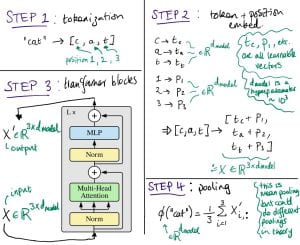
See Figure 2 for an illustration of how a transformer encoder calculates an embedding for a piece of text. In the figure we show how to encode “cat”, but we can encode arbitrary pieces of text in a similar way. The transformer block details are out of scope here; though, for these details I personally found Attention is All You Need [9] helpful, the crucial part being the Multi-Head Attention which allows modelling dependencies between words.

Figure 2: Transformer illustration (transformer block image taken from [6])
The transformer encoder is very flexible, with almost every component parameterized by a learnable weight / bias – this is why it can be used to model the complicated semantics in natural language. The pooling step in Figure 2, where we map our sequence embedding $X’$ to a fixed size, is not part of a ‘regular’ transformer, but it is essential for us. It ensures that our score function $\langle \phi(q), \phi(d) \rangle$ will work when $q$ and $d$ have different sizes.
Making the score function good for search
There is a massive issue with transformer embedding as described above, at least for our purposes – there is no reason to believe it will satisfy simple semantic properties, such as,
$\text{score}(\text{“busy place”}, \text{“tokyo”}) > \text{score}(\text{“busy place”}, \text{“a small village”})$
‘But why would the above not work?’ Because, of course, transformers are typically trained to predict the next token in a sequence, not to differentiate pieces of text according to their semantics.
The solution to this problem is not to eschew transformer embeddings, but rather to fine-tune them for search. The idea is to encourage the transformer to give us embeddings that place semantically dissimilar items far apart. E.g. let $q=$’busy place’, then we want $ d^+=$’tokyo’ to be close to $q$ and $d^-=$’a small village’ to be far away.
This semantic separation can be achieved by fine-tuning with a contrastive loss [1,2,3,10],
$$
\text{maximize}_{\theta}\,\mathcal{L} = \log \frac{\exp(\text{score}(q, d^+))}{\exp(\text{score}(q, d^+)) + \exp(\text{score}(q, d^-))},
$$
where $\theta$ represents the transformer parameters. The $\exp$’s in the contastive loss are to ensure we never divide by zero. Note that we can interpret the contrastive loss as doing classification since we can think of the argument to the logarithm as $p(d^+ | q)$.
That’s all we need, in principle, to turn a transformer encoder into a text embedder! In practice, the contrastive loss can be generalized to include more positive and negative examples, and it is indeed a good idea to have a large batch size [11] (intuitively it makes the separation of positive and negative examples more difficult, resulting in a better classifier). We also need a fine-tuning dataset – a dataset of positive/negative examples. OpenAI showed that it is possible to construct one in an unsupervised fashion [1]. However, there are also publicly available datasets for supervised fine-tuning, e.g. MSMARCO [12].
Extensions
One really interesting avenue of research is training of general purposes encoders. The idea is to provide instructions alongside the queries/documents [2,3]. The instruction could be $\verb|Embed this document for search: {document}|$ (for the application we’ve been discussing), or $\verb|Embed this document for clustering: {document}|$ to get embeddings suitable for clustering, or $\verb|Embed this document for sentiment analysis: {document}|$ for embeddings suitable for sentiment analysis. The system is fine-tuned end-to-end with the appropriate task, e.g. a contrastive learning objective for the search instruction, a classification objective for sentiment analysis, etc., leaving us with an easy way to generate embeddings for different tasks.
A note on scaling
The real power of semantic (and keyword) search comes when a search corpus is too large for a human to search manually. However if the corpus is enormous, we’d rather avoid looking at every document each time we get a query. Thankfully, there are methods to avoid this by using specially tailored data structures: see Inverted Indices for keyword algorithms, and Hierarchical Navigable Small World graphs [5] for semantic algorithms. These both reduce search time complexity from $\mathcal{O}(|\mathcal{D}|)$ to $\mathcal{O}(\log |\mathcal{D}|)$, where $|\mathcal{D}|$ is the corpus size.
There are many startups (Pinecone, Weviate, Milvus, Chroma, etc.) that are proposing so-called vector databases – databases in which embeddings are stored, and queries can be efficiently performed. Though, there is also work contesting the need for these types of database in the first place [7].
Summary
We summarised search, semantic search, and how transformers are fine-tuned for search with a contrastive loss. I personally find this a very nice area of research with exciting real-world applications – please reach out (ben.anson@bristol.ac.uk) if you’d like to discuss it!
References
[1]: Text and code embeddings by contrastive pre-training, Neelakantan et al (2022)
[2]: Task-aware Retrieval with Instructions, Asai et al (2022)
[3]: One embedder, any task: Instruction-finetuned text embeddings, Su et al (2022)
[4]: Some simple effective approximations to the 2-poisson model for probabilistic weighted retrieval, Robertson and Walker (1994)
[5]: Efficient and robust approximate nearest neighbor search using Hierarchical Navigable Small World graphs, https://arxiv.org/abs/1603.09320
[6]: An Image is Worth 16×16 Words: Transformers for Image Recognition at Scale, https://arxiv.org/abs/2010.11929
[7]: Vector Search with OpenAI Embeddings: Lucene Is All You Need, arXiv preprint arXiv:2308.14963
[8]: Complement lexical retrieval model with semantic residual embeddings, Advances in Information Retrieval (2021)
[9]: Attention is all you need, Advances in neural information processing systems (2017)
[10]: Sgpt: Gpt sentence embeddings for semantic search, arXiv preprint arXiv:2202.08904
[11]: Contrastive representation learning: A framework and review, IEEE Access 8 (2020)
[12]: Ms marco: A human generated machine reading comprehension dataset, arXiv preprint arXiv:1611.09268
[13]: AdANNS: A Framework for Adaptive Semantic Search, arXiv preprint arXiv:2305.19435

