Student Perspectives: Density Ratio Estimation with Missing Data

A post by Josh Givens, PhD student on the Compass programme.

Density ratio estimation is a highly useful field of mathematics with many applications.  This post describes my research undertaken alongside my supervisors Song Liu and Henry Reeve which aims to make density ratio estimation robust to missing data. This work was recently published in proceedings for AISTATS 2023.

Density Ratio Estimation

Definition

As the name suggests, density ratio estimation is simply the task of estimating the ratio between two probability densities. More precisely for two RVs (Random Variables) Z^0, Z^1 on some space \mathcal{Z} with probability density functions (PDFs) p_0, p_1 respectively, the density ratio is the function r^*:\mathcal{Z}\rightarrow\mathbb{R} defined by

r^*(z):=\frac{p_0(z)}{p_1(z)}.

Plot of the scaled density ratio alongside the PDFs for the two classes.

Density ratio estimation (DRE) is then the practice of using IID (independent and identically distributed) samples from Z^0 and Z^1 to estimate r^*. What makes DRE so useful is that it gives us a way to characterise the difference between these 2 classes of data using just 1 quantity, r^*.


The Density Ratio in Classification

We now give demonstrate this characterisability in the case of classification. To frame this as a classification problem define Y\sim\text{Bernoulli}(0.5) and Z by Z|Y=y\sim Z^{y}. The task of predicting Y given Z using some function \phi:\mathcal{Z}\rightarrow\{0,1\} is then our standard classification problem. In classification a common target is the Bayes Optimal Classifier, the classifier \phi^* which maximises \mathbb{P}(Y=\phi(Z)). We can write this classifier in terms of r^*  as we know that \phi^*(z)=\mathbb{I}\{\mathbb{P}(Y=1|Z=z)>0.5\} where \mathbb{I} is the indicator function. Then, by the total law of probability, we have

\mathbb{P}(Y=1|Z=z)=\frac{p_{Z|Y=1}(z)\mathbb{P}(Y=1)}{p_{Z|Y=1}(z)\mathbb{P}(Y=1)+p_{Z|Y=0}(z)\mathbb{P}(Y=0)}

=\frac{p_1(z)\mathbb{P}(Y=1)}{p_1(z)\mathbb{P}(Y=1)+p_0(z)\mathbb{P}(Y=0)} =\frac{1}{1+\frac{1}{r}\frac{\mathbb{P}(Y=0)}{\mathbb{P}(Y=1)}}.

Hence to learn the Bayes optimal classifier it is sufficient to learn the density ratio and a constant. This pattern extends well beyond Bayes optimal classification to many other areas such as error controlled classification, GANs, importance sampling, covariate shift, and others.  Generally speaking, if you are in any situation where you need to characterise the difference between two classes of data, it’s likely that the density ratio will make an appearance.

Estimation Implementation – KLIEP

Now we have properly introduced and motivated DRE, we need to look at how we can go about performing it. We will focus on one popular method called KLIEP here but there are a many different methods out there (see Sugiyama et al 2012 for some additional examples.)

The intuition behind KLIEP is simple: as r^* \cdot p_0=p_1, if \hat r\cdot p_0 is “close” to p_1 then \hat r is a good estimate of r^*. To measure this notion of closeness KLIEP uses the KL (Kullback-Liebler) divergence which measures the distance between 2 probability distributions. We can now formulate our ideal KLIEP objective as follows:

\underset{r}{\text{min}}~ KL(p_1|p_0\cdot r)

\text{subject to:}~ \int_{\mathcal{Z}}r(z)p_0(z)\mathrm{d}z=1

where KL(p|p') represent the KL divergence from p to p'. The constraint  ensures that the right hand side of our KL divergence is indeed a PDF. From the definition of the KL-divergence we can rewrite the solution to this as \hat r:=\frac{\tilde r}{\mathbb{E}[r(X^0)]} where \tilde r is the solution to the unconstrained optimisation

\underset{r}{\text{min}}~\mathbb{E}[\log (r(Z^1))]-\log(\mathbb{E}[r(Z^0)]).

As this is now just an unconstrained optimisation over expectations of known transformations of Z^0, Z^1, we can approximate this using samples. Given samples z^0_1,\dotsc,z^0_n from Z_0 and samples z^1_1,\dotsc,z^1_n from Z_1 our estimate of the density ratio will be \hat r:=\left(\frac{1}{n}\sum_{i=1}^nr(z_i^0)\right)^{-1}\tilde r  where \tilde r solves

\underset{r}{\min}~ \frac{1}{n}\sum_{i=1}^n \log(r(z^1_i))-\log\left(\frac{1}{n}\sum_{i=1}^n r(z^0_i)\right).

Despite KLIEP being commonly used, up until now it has not been made robust to missing not at random data. This is what our research aims to do.

Missing Data

Suppose that instead of observing samples from Z, we observe samples from some corrupted version of Z, X. We assume that \mathbb{P}(\{X=\varnothing\}\cup \{X=Z\})=1 so that either X is missing or X takes the value of Z. We also assume that whether X is missing depends upon the value of Z. Specifically we assume \mathbb{P}(X=\varnothing|Z=z)=\varphi(z) with \varphi(z) not constant and refer to \varphi as the missingness function. This type of missingness is known as missing not at random (MNAR) and when dealt with improperly can lead to biased result. Some examples of MNAR data could be readings take from a medical instrument which is more likely to err when attempting to read extreme values or recording responses to a questionnaire where respondents may be more likely to not answer if the deem their response to be unfavourable. Note that while we do not see what the true response would be, we do at least get a response meaning that we know when an observation is missing.

Missing Data with DRE

We now go back to density ratio estimation in the case where instead of observing samples from  Z^0,Z^1  we observe samples from their corrupted versions X^0, X^1. We take their respective missingness functions to be \varphi_0, \varphi_1 and assume them to be known. Now let us look at what would happen if we implemented KLIEP with the data naively by simply filtering out the missing-values. In this case, the actual density ratio we would be estimating would be

r'(z)
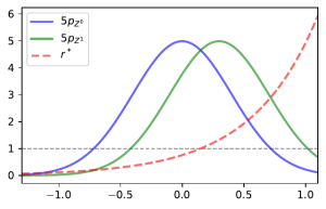
:=\frac{p_{X_1|X_1\neq\varnothing}(z)}{p_{X_0|X_o\neq\varnothing}(z)}\propto\frac{(1-\varphi_1(z))p_1(z)}{(1-\varphi_0(z))p_0(z)}\not{\propto}r^*(z)

and so we would get inaccurate estimates of the density ratio no matter how many samples are used to estimate it. The image below demonstrates this in the case were samples in class 1 are more likely to be missing when larger and class 0 has no missingness.

A plot of the density ratio using both the full data and only the observed part of the corrupted data

Our Solution

Our solution to this problem is to use importance weighting. Using relationships between the densities of X and Z we have that

\mathbb{E}[g(Z)]=\mathbb{E}\left[\frac{\mathbb{I}\{X\neq\varnothing\}g(X)}{1-\varphi(X)}\right].

As such we can re-write the KLIEP objective to keep our expectation estimation unbiased even when using these corrupted samples. This gives our modified objective which we call M-KLIEP as follows. Given samples x^0_1,\dotsc,x^0_n from X_0 and samples x^1_1,\dotsc,x^1_n from X_1 our estimate is \hat r=\left(\frac{1}{n}\sum_{i=1}^n\frac{\mathbb{I}\{x_i^0\neq\varnothing\}r(x_i^0)}{1-\varphi_o(x_i^o)}\right)^{-1}\tilde r where \tilde r solves

\underset{r}{\min}~\frac{1}{n}\sum_{i=1}^n\frac{\mathbb{I}\{x_i^1\neq\varnothing\}\log(r(x_i^1))}{1-\varphi_1(x_i^1)}-\log\left(\frac{1}{n}\sum_{i=1}^n\frac{\mathbb{I}\{x_i^0\neq\varnothing\}r(x_i^0)}{1-\varphi_0(x_i^0)}\right).

This objective will now target r^* even when used on MNAR data.

Application to Classification

We now apply our density ratio estimation on MNAR data to estimate the Bayes optimal classifier. Below shows a plot of samples alongside the true Bayes optimal classifier and estimated classifiers from the samples via our method M-KLIEP and a naive method CC-KLIEP which simply ignores missing points. Missing data points are faded out.

Faded points represent missing values. M-KLIEP represents our method, CC-KLIEP represents a Naive approach, BOC gives the Bayes optimal classifier

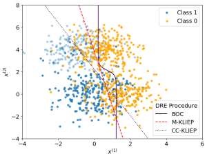
As we can see, due to not accounting for the MNAR nature of the data, CC-KLIEP underestimates the true number of class 1 samples in the top left region and therefore produces a worse classifier than our approach.

Additional Contributions

As well as this modified objective our paper provides the following additional contributions:

  • Theoretical finite sample bounds on the accuracy of our modified procedure.
  • Methods for learning the missingness functions \varphi_1,\varphi_0.
  • Expansions to partial missingness via a Naive-Bayes framework.
  • Downstream implementation of our method within Neyman-Pearson classification.
  • Adaptations to Neyman-Pearson classification itself making it robust to MNAR data.

For more details see our paper and corresponding github repository. If you have any questions on this work feel free to contact me at josh.givens@bristol.ac.uk.

References

Givens, J., Liu, S., & Reeve, H. W. J. (2023). Density ratio estimation and neyman pearson classification with missing data. In F. Ruiz, J. Dy, & J.-W. van de Meent (Eds.), Proceedings of the 26th international conference on artificial intelligence and statistics (Vol. 206, pp. 8645–8681). PMLR.
Sugiyama, M., Suzuki, T., & Kanamori, T. (2012). Density Ratio Estimation in Machine Learning. Cambridge University Press.

Compass students attending AISTATS 2023 in Valencia

We (Ed Davis, Josh Givens, Alex Modell, and Hannah Sansford) attended the 2023 AISTATS conference in Valencia in order to explore the interesting research being presented as well as present some of our own work. While we talked about our work being published at the conference in this earlier blog post, having now attended the conference, we thought we’d talk about our experience there. We’ll spotlight some of the talks and posters which interested us most and talk about our highlights of Valencia as a whole.

Talks & Posters

Mode-Seeking Divergences: Theory and Applications to GANs

One especially interesting talk and poster at the conference was presented by Cheuk Ting Li on their work in collaboration with Farzan Farnia. This work aims to set up a formal classification for various probability measure divergences (such as f-Divergences, Wasserstein distance, etc.) in terms of there mode-seeking or mode-covering properties. By mode-seeking/mode-covering we mean the behaviour of the divergence when used to fit a unimodal distribution to a multi-model target. Specifically a mode-seeking divergence will encourage the target distribution to fit just one of the modes ignoring the other while a mode covering divergence will encourage the distribution to cover all modes leading to less accurate fitting on an individual mode but better covering the full support of the distribution. While these notions of mode-seeking and mode-covering divergences had been discussed before, up to this point there seems to be no formal definition for these properties, and disagreement on the appropriate categorisation of some divergences. This work presents such a definition and uses it to categorise many of the popular divergence methods. Additionally they show how an additive combination a mode seeking f-divergence and the 1-Wasserstein distance retain the mode-seeking property of the f-divergence while being implementable using only samples from our target distribution (rather than knowledge of the distribution itself) making it a desirable divergence for use with GANs.

Talk: https://youtu.be/F7LdHIzZQow

Paper: https://proceedings.mlr.press/v206/ting-li23a.html

Using Sliced Mutual Information to Study Memorization and Generalization in
Deep Neural Networks

The benefit of attending large conferences like AISTATS is having the opportunity to hear talks that are not related to your main research topic. This was the case with a talk by Wongso et. al. was one such talk. Although it did not overlap with any of our main research areas, we all found this talk very interesting.
The talk was on the topic of tracking memorisation and generalisation in deep neural networks (DNNs) through the use of /sliced mutual information/. Mutual information (MI) is commonly used in information theory and represents the reduction of uncertainty about one random variable, given the knowledge of the other. However, MI is hard to estimate in high dimensions, which makes it a prohibitive metric for use in neural networks.
Enter sliced mutual information (SMI). This metric is the average of the MI terms between their one-dimensional projections. The main difference between SMI and MI is that SMI is scalable to high dimensions and scales faster than MI.
Next, let’s talk about memorisation. Memorisation is known to occur in DNNs and is where the DNN fits random labels in training as it has memorised noisy labels in training, leading to bad generalisation. The authors demonstrate this behaviour by fitting a multi-layer perceptron to the MNIST dataset with various amounts of label noise. As the noise increased, the difference between the training and test accuracy became greater.
As the label noise increases, the MI between the features and target variable does not change, meaning that MI did not track the loss in generalisation. However, the authors show that the SMI did track the generalisation. As the label noise increased, the SMI decreased significantly as the MLP’s generalisation got worse. Their main theorem showed that SMI is lower-bounded by a term which includes the spherical soft-margin separation, a quantity which is used to track memorisation and generalisation!
In summary, unlike MI, SMI can track memorization and generalisation in DNNs. If you’d like to know more, you can find the full paper here: https://proceedings.mlr.press/v206/wongso23a.html.

Invited Speakers and the Test of Time Award

As well as the talks on papers that had been selected for oral presentation, each day began with a (longer) invited talk which, for many of us, were highlights of each day. The invited speakers were extremely engaging and covered varied and interesting topics; from Arthur Gretton (UCL) presenting ‘Causal Effect Estimation with Context and Confounders’ to Shakir Mohamed (DeepMind) presenting ‘Elevating our Evaluations: Technical and Sociotechnical Standards of Assessment in Machine Learning’. A favourite amongst us was a talk from Tamara Broderick (MIT) titled ‘An Automatic Finite-Sample Robustness Check: Can Dropping a Little Data Change Conclusions?’. In this talk she addressed a worry that researchers might have when the goal is to analyse a data sample and apply any conclusions to a new population: was a small proportion of the data sample instrumental to the original conclusion? Tamara and collorators propose a method to assess the sensitivity of statistical conclusions to the removal of a very small fraction of the data set. They find that sensitivity is driven by a signal-to-noise ratio in the inference problem, does not disappear asymptotically, and is not decided by misspecification. In experiments they find that many data analyses are robust, but that the conclusions of severeal influential economics papers can be changed by removing (much) less than 1% of the data! A link to the talk can be found here: https://youtu.be/QYtIEqlwLHE

This year, AISTATS featured a Test of Time Award to recognise a paper from 10 years ago that has had a prominent impact in the field. It was awarded to Andreas Damianou and Neil Lawrence for the paper ‘Deep Gaussian Processes’, and their talk was a definite highlight of the conferece. Many of us had seen Neil speak at a seminar at the University of Bristol last year and, being the engaging speaker he is, we were looking forward to hearing him speak again. Rather than focussing on the technical details of the paper, Neils talk concentrated on his (and the machine learning community’s) research philosophy in the years preceeding writing the paper, and how the paper came about – a very interesting insight, and a refreshing break from the many technical talks!

Valencia

There was so much to like about Valencia even from our short stay there. We’ll try and give you a very brief highlight of our favourite things.

Food & Drink:

Obviously Valencia is renowned for being the birthplace of paella and while the paella was good we sampled many other delights our stay. Our collective highlight was the nicest Burrata any of us had ever had which, in a stunning display of individualism, all four of us decided to get on our first day at the conference.

Artist rendition of our 4 meals.

Beach:

About half an hours tram ride from the conference centre are the beaches of Valencia. These stretch for miles as well as having a good 100m in depth with (surprisingly hot) sand covering the lot. We visited these after the end of the conference on the Thursday and despite it being the only cloudy day of the week it was a perfect way to relax at the end of a hectic few days with the pleasantly temperate water being an added bonus.

Architecture:

Valencia has so much interesting architecture scattered around the city centre. One of the most memorable remarkable places was the San Nicolás de Bari and San Pedro Mártir (Church of San Nicolás) which is known as the Sistine chapel of Valencia (according to the audio-guide for the church at least) with its incredible painted ceiling and live organ playing.

Ceiling of the Church of San Nicolás


Skip to toolbar