A post by Sam Stockman, PhD student on the Compass programme.

Introduction

Throughout my PhD I aim to bridge a gap between advances made in the machine learning community and the age-old problem of earthquake forecasting. In this cross-disciplinary work with Max Werner from the School of Earth Sciences and Dan Lawson from the School of Mathematics, I hope to create more powerful, efficient and robust models for forecasting, that can make earthquake prone areas safer for their inhabitants.

For years seismologists have sought to model the structure and dynamics of the earth in order to make predictions about earthquakes. They have mapped out the structure of fault lines and conducted experiments in the lab where they submit rock to great amounts of force in order to simulate plate tectonics on a small scale. Yet when trying to forecast earthquakes on a short time scale (that’s hours and days, not tens of years), these models based on the knowledge of the underlying physics are regularly outperformed by models that are statistically motivated. In statistical seismology we seek to make predictions through looking at distributions of the times, locations and magnitudes of earthquakes and use them to forecast the future.

The most popular way to model earthquakes is to consider them to be realisations of a Point Process. These are statistical models that generate discrete sequences of the times $\{t_i\}_{i=1}^n$ with magnitudes $\{m_i\}_{i=1}^n$ . For simplicity let us ignore any idea of where these earthquakes are located in what follows. Point Processes are described by their intensity function,

$\lambda(t|H_t)dt = \mathbb{P}\left(\text{Earthquake} \in [t,t+dt]|H_t\right).$

Which is the probability of observing an earthquake in a small interval at time $t$ conditional on the history of all the earthquakes before $t$ , denoted $H_t$ . The most popular Point Process model for earthquakes is the Epidemic Type Aftershock Sequence (ETAS) model [1] with intensity function,

$\lambda(t|H_t)= \mu + \sum_{i:t_i<t}k(m_i)g(t-t_i).$

In this model, the rate of an earthquake occurrence is given by some base rate $\mu$ plus a contribution from summing over all the events before time $t$ . We can find the parameters in the intensity function through numerically maximising the likelihood of observing a sequence of earthquakes,

$\log L(\{t_i\}_{i=1}^n) = \sum_{i=1}^n \log \lambda(t_i|H_{t_i}) - \int_{t_{i-1}}^{t_i} \lambda(t|H_t)dt.$

Neural Point Processes [2]

In my work I seek to make improvements upon the ETAS model by moving away from defining a functional form for the intensity function. We do this through instead using a neural network, but not by directly modelling the intensity function as its output. We first model the intensity function as a function of the time since the last event $t_i$ and an approximation $\textbf{h}_i$ of the history of the Point Process,

$\lambda(t|H_t) = \phi(t-t_i,\textbf{h}_i).$

Then we let the output of our neural network be defined,

$\Phi(\tau_i,\textbf{h}_i) = \int_0^{\tau_i} \phi(s,\textbf{h}_i)ds.$

In doing this, it means that we can rewrite the likelihood equation,

$\log L(\{t_i\}_{i=1}^n) = \sum_{i=1}^n \log \lambda(t_i|H_{t_i}) - \int_{t_{i-1}}^{t_i} \lambda(t|H_t)dt$

$= \sum_{i=1}^n \left[ \log \frac{\partial}{\partial \tau_i}\Phi(\tau_i,\textbf{h}_i ) - \Phi(\tau_i,\textbf{h}_i)\right].$

This equation then becomes something that can be efficiently calculated using a neural network. Automatic differentiation allows us to calculate the derivative of the output of a network with respect to an input and thus rewriting the equation this way avoids us having to numerically calculate the integral that was there previously.

Experiments

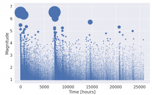
We can first test whether we can model earthquake data sufficiently well with this Neural Point Process by simulating data from the ETAS model. On fitting to this simulated data we can see that the Neural model is able to approximate the ETAS intensity function rather well.

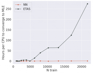
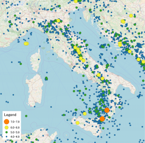
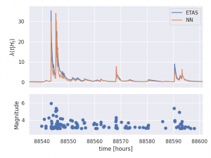
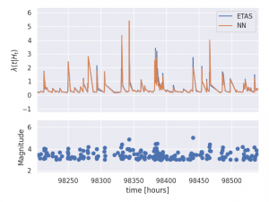
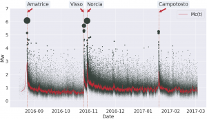
What is most promising is that we make serious improvements to the computational efficiency of training the point process. With ETAS, since there is a double sum in the likelihood, evaluating it grows like $O(N^2)$ with the size of the training dataset. The Neural model however, through approximating the history $H_t$ with the vector $\textbf{h}_i$ , only grows like $O(N)$ . This approximation of the history is done through learning an embedding of only the past $d$ earthquakes before time $t$ , $\textbf{h}_i = g(t_{i-d}, \dots , t_i)$ .

We can now compare both of these forecasting models on data from the series of large earthquakes that struck central Italy in 2016 [3]. One particular feature of this dataset along with all other seismic datasets is that following large earthquakes, due to the fact that the earth is shaking so much, we fail to record many of the small earthquakes that are occurring at the same time. Therefore not only do we have missing data, but the amount of missing data varies in time. 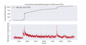This can be illustrated by the red line $Mc(t)$ , which is an estimate of the magnitude above which we have complete data.

We can compare the performance of the two models by looking at the cumulative difference in their likelihood score across the time spanned by the last three large earthquakes. Comparing this against the estimate for how complete the dataset is over time, we can see that the moments where the Neural model makes the most gain over ETAS is in fact the times at which the dataset is missing the most earthquakes.

Conclusion

These early results on flexible point process models for earthquakes demonstrate their potential for operational forecasting in areas of high seismic activity. What is most promising is that the model we have constructed is both more computationally efficient than ETAS as well as more robust to missing data following large earthquakes. Yet their effectiveness needs much more testing on a variety of real datasets from around the world. What is also needed, is a model that can also forecast earthquake’s location as well as time. But, these early results only encourage exploration in these directions.

References

[1] Y. Ogata. Statistical models for earthquake occurrences and residual analysis for point processes. Journal of the American Statistical association, 83(401):9–27, 1988.

[2] T. Omi, n. ueda, and K. Aihara. Fully neural network based model for general temporal point processes. In H. Wallach, H. Larochelle, A. Beygelzimer,
F. d’Alch ́e-Buc, E. Fox, and R. Garnett, editors, Advances in Neural Infor-
mation Processing Systems, volume 32, pages 2122–2132. Curran Associates,
Inc., 2019.

[3] Y. J. Tan, F. Waldhauser, W. L. Ellsworth, M. Zhang, W. Zhu, M. Michele, L. Chiaraluce, G. C. Beroza, and M. Segou. Machine-learning-based high-resolution earthquake catalog reveals how complex fault structures were activated during the 2016–2017 central italy sequence. The Seismic Record, 1(1):11–19, 2021.