QGAMs – Compass Blog

A post by Ben Griffiths, PhD student on the Compass programme.

My area of research is studying Quantile Generalised Additive Models (QGAMs), with my main application lying in energy demand forecasting. In particular, my focus is on developing faster and more stable fitting methods and model selection techniques. This blog post aims to briefly explain what QGAMs are, how to fit them, and a short illustrative example applying these techniques to data on extreme rainfall in Switzerland. I am supervised by Matteo Fasiolo and my research is sponsored by Électricité de France (EDF).

Quantile Generalised Additive Models

QGAMs are essentially the result of combining quantile regression (QR; performing regression on a specific quantile of the response) with a generalised additive model (GAM; fitting a model assuming additive smooth effects). Here we are in the regression setting, so let $F(y| \boldsymbol{x})$ be the conditional c.d.f. of a response, $y$ , given a $p$ -dimensional vector of covariates, $\boldsymbol{x}$ . In QR we model the $\tau$ th quantile, that is, $\mu_\tau(\boldsymbol{x}) = \inf \{y : F(y|\boldsymbol{x}) \geq \tau\}$ .

Examples of true quantiles of SHASH distribution.

This might be useful in cases where we do not need to model the full distribution of $y| \boldsymbol{x}$ and only need one particular quantile of interest (for example urban planners might only be interested in estimates of extreme rainfall e.g. $\tau = 0.95$ ). It also allows us to make no assumptions about the underlying true distribution, instead we can model the distribution empirically using multiple quantiles.

We can define the $\tau$ th quantile as the minimiser of expected loss

$L(\mu| \boldsymbol{x}) = \mathbb{E} \left\{\rho_\tau (y - \mu)| \boldsymbol{x} \right \} = \int \rho_\tau(y - \mu) d F(y|\boldsymbol{x}),$

w.r.t. $\mu = \mu_\tau(\boldsymbol{x})$ , where

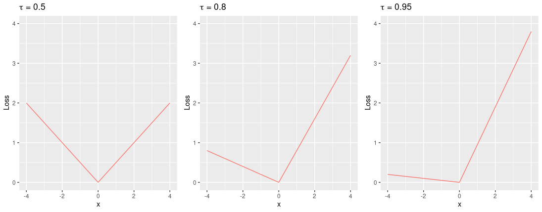
$\rho_\tau (z) = (\tau - 1) z \boldsymbol{1}(z<0) + \tau z \boldsymbol{1}(z \geq 0),$

is known as the pinball loss (Koenker, 2005).

Pinball loss for quantiles 0.5, 0.8, 0.95.

We can approximate the above expression empirically given a sample of size $n$ , which gives the quantile estimator, $\hat{\mu}_\tau(\boldsymbol{x}) = \boldsymbol{x}^\mathsf{T} \hat{\boldsymbol{\beta}}$ where

$\hat{\boldsymbol{\beta}} = \underset{\boldsymbol{\beta}}{\arg \min} \frac{1}{n} \sum_{i=1}^n \rho_\tau \left\{y_i - \boldsymbol{x}_i^\mathsf{T} \boldsymbol{\beta}\right\},$

where $\boldsymbol{x}_i$ is the $i$ th vector of covariates, and $\boldsymbol{\beta}$ is vector of regression coefficients.

So far we have described QR, so to turn this into a QGAM we assume $\mu_\tau(\boldsymbol{x})$ has additive structure, that is, we can write the $\tau$ th conditional quantile as

$\mu_\tau(\boldsymbol{x}) = \sum_{j=1}^m f_j(\boldsymbol{x}),$

where the $m$ additive terms are defined in terms of basis functions (e.g. spline bases). A marginal smooth effect could be, for example

$f_j(\boldsymbol{x}) = \sum_{k=1}^{r_j} \beta_{jk} b_{jk}(x_j),$

where $\beta_{jk}$ are unknown coefficients, $b_{jk}(x_j)$ are known spline basis functions and $r_j$ is the basis dimension.

Denote $\boldsymbol{\mathrm{x}}_i$ the vector of basis functions evaluated at $\boldsymbol{x}_i$ , then the $n \times d$ design matrix $\boldsymbol{\mathrm{X}}$ is defined as having $i$ th row $\boldsymbol{\mathrm{x}}_i$ , for $i = 1, \dots, n$ , and $d = r_1+\dots +r_m$ is the total basis dimension over all $f_j$ . Now the quantile estimate is defined as $\mu_\tau(\boldsymbol{x}_i) = \boldsymbol{\mathrm{x}}_i^\mathsf{T} \boldsymbol{\beta}$ . When estimating the regression coefficients, we put a ridge penalty on $\boldsymbol{\beta}_{j}$ to control complexity of $f_j$ , thus we seek to minimise the penalised pinball loss

$V(\boldsymbol{\beta},\boldsymbol{\gamma},\sigma) = \sum_{i=1}^n \frac{1}{\sigma} \rho_\tau \left\{y_i - \mu(\boldsymbol{x}_i)\right\} + \frac{1}{2} \sum_{j=1}^m \gamma_j \boldsymbol{\beta}^\mathsf{T} \boldsymbol{\mathrm{S}}_j \boldsymbol{\beta},$

where $\boldsymbol{\gamma} = (\gamma_1,\dots,\gamma_m)$ is a vector of positive smoothing parameters, $1/\sigma>0$ is the learning rate and the $\boldsymbol{\mathrm{S}}_j$ ‘s are positive semi-definite matrices which penalise the wiggliness of the corresponding effect $f_j$ . Minimising $V$ with respect to $\boldsymbol{\beta}$ given fixed $\sigma$ and $\boldsymbol{\gamma}$ leads to the maximum a posteriori (MAP) estimator $\hat{\boldsymbol{\beta}}$ .

There are a number of methods to tune the smoothing parameters and learning rate. The framework from Fasiolo et al. (2021) consists in:

calibrating $\sigma$ by Integrated Kullback–Leibler minimisation
selecting $\boldsymbol{\gamma}|\sigma$ by Laplace Approximate Marginal Loss minimisation
estimating $\boldsymbol{\beta}|\boldsymbol{\gamma},\sigma$ by minimising penalised Extended Log-F loss (note that this loss is simply a smoothed version of the pinball loss introduced above)

For more detail on what each of these steps means I refer the reader to Fasiolo et al. (2021). Clearly this three-layered nested optimisation can take a long time to converge, especially in cases where we have large datasets which is often the case for energy demand forecasting. So my project approach is to adapt this framework in order to make it less computationally expensive.

Application to Swiss Extreme Rainfall

Here I will briefly discuss one potential application of QGAMs, where we analyse a dataset consisting of observations of the most extreme 12 hourly total rainfall each year for 65 Swiss weather stations between 1981-2015. This data set can be found in the R package gamair and for model fitting I used the package mgcViz.

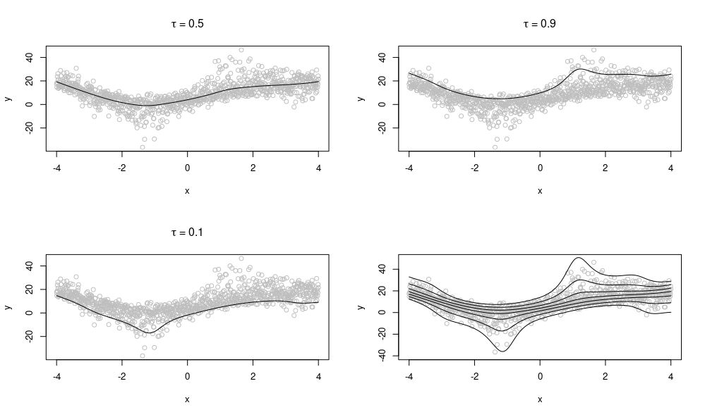
A basic QGAM for the 50% quantile (i.e. $\tau = 0.5$ ) can be fitted using the following formula

$\mu_i = \beta + \psi(\mathrm{reg}_i) + f_1(\mathrm{nao}_i) + f_2(\mathrm{el}_i) + f_3(\mathrm{Y}_i) + f_4(\mathrm{E}_i,\mathrm{N}_i),$

where $\beta$ is the intercept term, $\psi(\mathrm{reg}_i)$ is a parametric factor for climate region, $f_1, \dots, f_4$ are smooth effects, $\mathrm{nao}_i$ is the Annual North Atlantic Oscillation index, $\mathrm{el}_i$ is the metres above sea level, $\mathrm{Y}_i$ is the year of observation, and $\mathrm{E}_i$ and $\mathrm{N}_i$ are the degrees east and north respectively.

After fitting in mgcViz, we can plot the smooth effects and see how these affect the extreme yearly rainfall in Switzerland.

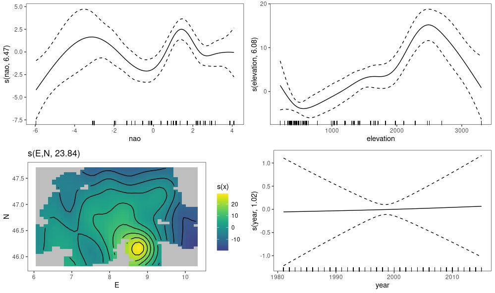
Fitted smooth effects for North Atlantic Oscillation index, elevation, degrees east and north and year of observation.

From the plots observe the following; as we increase the NAO index we observe a somewhat oscillatory effect on extreme rainfall; when increasing elevation we see a steady increase in extreme rainfall before a sharp drop after an elevation of around 2500 metres; as years increase we see a relatively flat effect on extreme rainfall indicating the extreme rainfall patterns might not change much over time (hopefully the reader won’t regard this as evidence against climate change); and from the spatial plot we see that the south-east of Switzerland appears to be more prone to more heavy extreme rainfall.

We could also look into fitting a 3D spatio-temporal tensor product effect, using the following formula

$\mu_i = \beta + \psi(\mathrm{reg}_i) + f_1(\mathrm{nao}_i) + f_2(\mathrm{el}_i) + t(\mathrm{E}_i,\mathrm{N}_i,\mathrm{Y}_i),$

where $t$ is the tensor product effect between $\mathrm{E}_i$ , $\mathrm{N}_i$ and $\mathrm{Y}_i$ . We can examine the spatial effect on extreme rainfall over time by plotting the smooths.

3D spatio-temporal tensor smooths for years 1985, 1995, 2005 and 2015.

There does not seem to be a significant interaction between the location and year, since we see little change between the plots, except for perhaps a slight decrease in the south-east.

Finally, we can make the most of the QGAM framework by fitting multiple quantiles at once. Here we fit the first formula for quantiles $\tau = 0.1, 0.2, \dots, 0.9$ , and we can examine the fitted smooths for each quantile on the spatial effect.

Spatial smooths for quantiles 0.1, 0.2, …, 0.9.

Interestingly the spatial effect is much stronger in higher quantiles than in the lower ones, where we see a relatively weak effect at the 0.1 quantile, and a very strong effect at the 0.9 quantile ranging between around -30 and +60.

The example discussed here is but one of many potential applications of QGAMs. As mentioned in the introduction, my research area is motivated by energy demand forecasting. My current/future research is focused on adapting the QGAM fitting framework to obtain faster fitting.

References

Fasiolo, M., S. N. Wood, M. Zaffran, R. Nedellec, and Y. Goude (2021). Fast calibrated additive quantile regression. Journal of the American Statistical Association 116 (535), 1402–1412.

Koenker, R. (2005). Quantile Regression. Cambridge University Press.

Tag: QGAMs

Student Perspectives: An Introduction to QGAMs

Quantile Generalised Additive Models

Application to Swiss Extreme Rainfall

References