A post by Edward Milsom, PhD student on the Compass programme.

This blog post provides a simple introduction to Deep Kernel Machines[1] (DKMs), a novel supervised learning method that combines the advantages of both deep learning and kernel methods. This work provides the foundation of my current research on convolutional DKMs, which is supervised by Dr Laurence Aitchison.

Why aren’t kernels cool anymore?

Kernel methods were once top-dog in machine learning due to their ability to implicitly map data to complicated feature spaces, where the problem usually becomes simpler, without ever explicitly computing the transformation. However, in the past decade deep learning has become the new king for complicated tasks like computer vision and natural language processing.

Neural networks are flexible when learning representations

The reason is twofold: First, neural networks have millions of tunable parameters that allow them to learn their feature mappings automatically from the data, which is crucial for domains like images which are too complex for us to specify good, useful features by hand. Second, their layer-wise structure means these mappings can be built up to increasingly more abstract representations, while each layer itself is relatively simple[2]. For example, trying to learn a single function that takes in pixels from pictures of animals and outputs their species is difficult; it is easier to map pixels to corners and edges, then shapes, then body parts, and so on.

Kernel methods are rigid when learning representations

It is therefore notable that classical kernel methods lack these characteristics: most kernels have a very small number of tunable hyperparameters, meaning their mappings cannot flexibly adapt to the task at hand, leaving us stuck with a feature space that, while complex, might be ill-suited to our problem.

To remedy this, a body of work exists that attempts to marry kernels with deep learning[3][4][5]. DKMs fall within this body of work. One way in which DKMs differ from previous work is that the model works solely with Gram matrices, rather than alternating between Gram matrices and feature vectors, which is what some methods choose to do instead.

Before we discuss DKMs, we should first recap kernel machines.

Kernel Machines

In standard kernel machines (i.e. Gaussian processes / kernel ridge regression) we can use training data $\mathbf X_{\text{train}} \in \mathbb R^{d_\text{input}},\mathbf Y_{\text{train}} \in \mathbb R^{d_\text{output}}$ , along with a kernel function $k(\cdot,\cdot):\mathbb R^{d_\text{input}} \times \mathbb R^{d_\text{input}} \rightarrow \mathbb R$ , to predict the output values for a new set of test inputs $\mathbf X_*$ :

$\mathbf F_* = \mathbf K_{*\text{t}} \mathbf K_{\text{tt}}^{-1} \mathbf Y_{\text{train}}$

where for shorthand we denote by $\mathbf K_{*\text{t}} \in \mathbb R^{N_* \times N}$ the kernel matrix comparing test to training points, and $\mathbf K_{\text{tt}} = \mathbf K(\mathbf X_{\text{train}}) \in \mathbb R^{N \times N}$ the training data kernel matrix (kernel matrices are computed by just applying the kernel function to all possible pairs of points).

Kernel functions are equivalent to transforming our datapoints using a feature map $\phi(\cdot):\mathbb R^{d_\text{input}} \rightarrow \mathbb R^{d_\phi}$ and then computing the inner product between them:

$\mathbf K(\mathbf X) = \mathbf \Phi(\mathbf X) \mathbf \Phi (\mathbf X)^T = \mathbf \Phi \mathbf \Phi^T$

where $\mathbf \Phi \in \mathbb R^{N \times d_\phi}$ is the matrix formed by applying $\phi$ to every datapoint in $\mathbf X$ . Crucially, we never compute $\mathbf \Phi$ (it is implicit) because we instead compute the kernel matrix with $k$ . The choice of $k$ determines what the implicit feature mapping $\phi$ is, which in some cases can be infinite-dimensional i.e. $d_\phi = \infty$ . This is possible since we never actually work with $\phi$ , only its inner product. This ability to implicitly use $\phi$ while only computing $\mathbf K$ is called the kernel trick. These feature mappings are often complicated, and can, for example, turn difficult classification problems into linearly separable ones.

Kernel machine rigidity

As we can see, the prediction for new points is simply a linear combination of the training $Y$ values, where the weights for this linear combination are given by the kernel. Loosely, more similar training datapoints (as judged by the kernel) have a greater contribution to the prediction on the test point.

Deep Kernels

As we discussed, the kernel defines an implicit feature mapping $\phi$ . Inspired by deep learning, can we create a deep kernel that applies $\phi$ multiple times?

$\mathbf G^l = \mathbf K^l(\mathbf X) := \mathbf \Phi ( \mathbf \Phi ( \cdots \mathbf \Phi(\mathbf X))) \mathbf \Phi ( \mathbf \Phi ( \cdots \mathbf \Phi(\mathbf X)))^T = \mathbf \Phi^l(\mathbf X) \mathbf \Phi^l(\mathbf X)^T$

This could explain why kernel machines struggle with complex data like images. While our kernel does give us a complex implicit feature map $\phi$ , this feature map is fixed (except for a few hyperparameters which we select during training). The practitioner must decide on (or create) a kernel which will be best suited for their problem. This is very difficult for complex data like images. Deep learning has shown us that if we want to perform well on these tasks, we must let the model learn its own representation.

(We introduce Gram matrix notation $\mathbf G^l$ as it will be useful later). For some kernels, yes we can! In order to compute $\mathbf K(\mathbf X)$ we usually need to have access to $\mathbf X$ . However it turns out that for many commonly used kernels, we can compute $\mathbf K(\mathbf X)$ while only knowing $\mathbf X \mathbf X^T$ . Since implicitly $\mathbf K = \mathbf \Phi \mathbf \Phi^T$ , it is therefore possible to apply $k$ again (implicitly using $\mathbf \Phi$ as the new inputs) and compute $\mathbf K^2(\mathbf X \mathbf X^T)$ .

Take, for example, the RBF kernel:

$k(\mathbf{x}_i, \mathbf{x}_j) = \exp\left(-\frac{\|\mathbf{x}_i - \mathbf{x}_j\|^2}{2\sigma^2}\right)$

To compute this kernel, we don’t actually need $\mathbf X$ : all we need to know is the squared distances between all pairs of data points, which can be computed using $\mathbf G^0 := \mathbf X \mathbf X^T$ :

$\begin{aligned} \|\mathbf{x}_i - \mathbf{x}_j\|^2 &:= \sum_{\lambda=1}^{d_\text{input}}(x_{i\lambda} - x_{j\lambda})^2\\ &= \sum_{\lambda=1}^{N_l} x_{i\lambda}^2 -2x_{i\lambda}x_{j\lambda} + x_{j\lambda}^2\\ &= G_{ii}^0 - 2 G_{ij}^0 + G_{jj}^0. \end{aligned}$

Hence, starting from $\mathbf G^0 = \mathbf X \mathbf X^T$ , we can compute a deep kernel via

$\mathbf G^l = \underbrace{\mathbf K( \mathbf K( \cdots \mathbf K(}_{l \text{ times}} \mathbf G^0))).$

This is very nice, but it doesn’t actually solve our original problem! Each layer is still a rigid transformation with only a few hyperparameters to allow it to adapt to data. In order to mimic deep learning, we need to somehow allow more flexibility. This is where Deep Kernel Machines come in.

Deep Kernel Machines

We could write the above deep kernel formulation recursively as

$\mathbf G^l = \mathbf K( \mathbf G^{l-1}).$

which simply says each layer is equal to the kernel applied to the previous layer. This transformation is too rigid, so to solve this, a Deep Kernel Machine does not force $\mathbf G^l$ to be equal to $\mathbf K (\mathbf G^{l-1})$ , but instead just encourages them to be close. It does this by optimising the gram matrices $\mathbf G^l$ over an objective function, called the DKM objective.

If this idea seems a little strange, just remember that “training” in kernel machines simply means computing your Gram (kernel) matrix from the training data. We are doing the same thing (albeit for multiple layers) except that instead of computing our Gram matrices using a fixed kernel function $k$ , we compute them by minimising an objective.

The DKM objective

The DKM objective function is defined as

$\mathcal L (\mathbf G^1,\dots,\mathbf G^L) = \log P(\mathbf Y | \mathbf G^L) - \sum_{l=1}^L \nu_l D_{\text{KL}}\left(\mathcal{N}(\mathbf{0},\mathbf G^l) || \mathcal{N}(\mathbf{0},\mathbf K(\mathbf G^{l-1})\right)$

assuming we have $L$ layers. In the original paper, the DKM objective was derived from a variational inference argument on an infinite-width deep Gaussian process, but the resulting expression is intuitive enough that it could plausibly have been invented independently. It has 2 terms, which simply state that the likelihood of our data according to the final output of our model should be maximised (first term), and that our Gram matrices should smoothly interpolate between the layers (second term).

The first term therefore encourages good predictive performance, while the second term acts as a regulariser: it is minimised when our inducing Gram matrices are equal to the kernel matrices from the previous layer, which is to say that no flexibility is added over a deep kernel. The $\nu_l$ constants are hyperparameters that control how strong each layer’s regularisation is compared to the likelihood term.

By the way, notice how we still compute the kernel $\mathbf K(\mathbf G^{l-1})$ so that we know how close we are to the deep kernel.

DKM Prediction

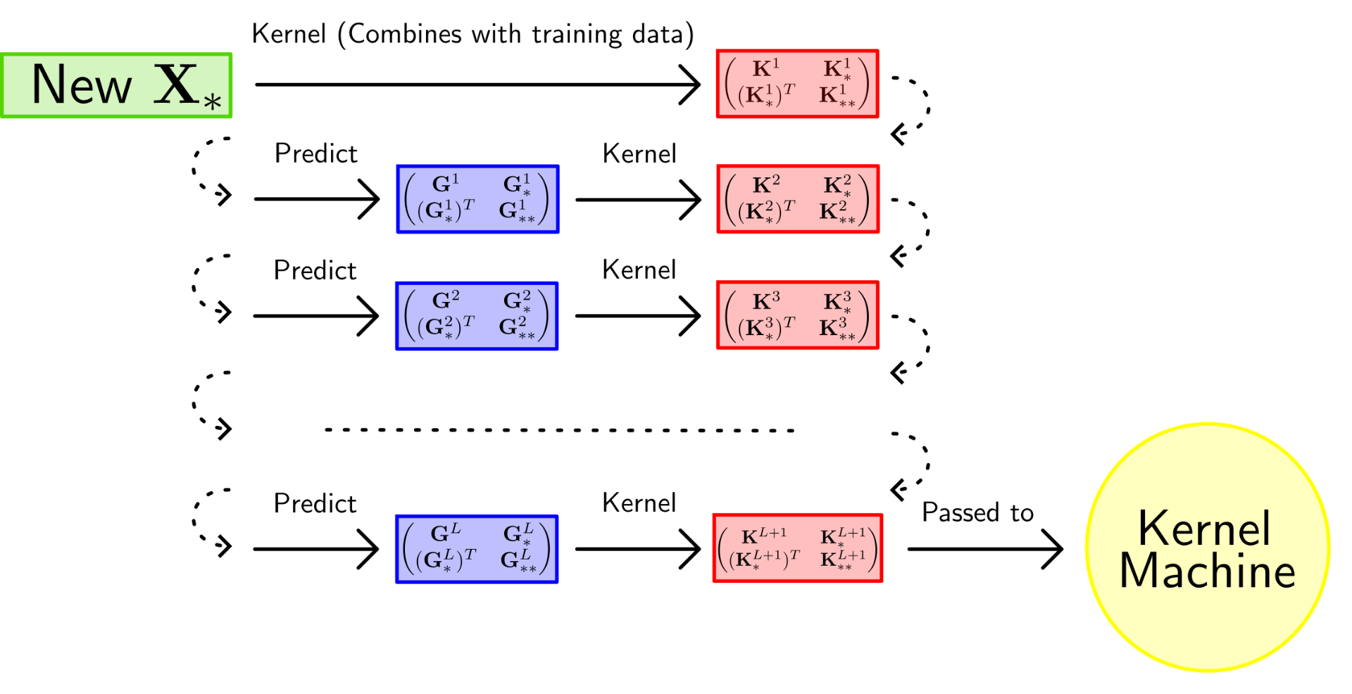
Suppose we’ve optimised our Gram matrices and we now wish to predict the output values for a new set of test inputs $\mathbf X_*$ . Like with regular kernel methods, we need to concatenate our test points to our training points to create block matrices that represent the joint between training and test:

$\begin{pmatrix} \mathbf X_t \\ \mathbf X_* \end{pmatrix}$

$\begin{pmatrix} \mathbf G^l & \mathbf G_{*}^l\\ (\mathbf G_{*}^l)^T & \mathbf G_{**}^l \end{pmatrix}$

$\begin{pmatrix} \mathbf K^{l+1} & \mathbf K_{*}^{l+1}\\ (\mathbf K_{*}^{l+1})^T & \mathbf K_{**}^{l+1} \end{pmatrix} := \mathbf K \begin{pmatrix} \mathbf G^{l} & \mathbf G_{*}^{l}\\ (\mathbf G_{*}^{l})^T & \mathbf G_{**}^{l} \end{pmatrix}$

where $\mathbf X_t \in \mathbb R^{N\times d_\text{input}}, \mathbf X_* \in \mathbb R^{N_* \times d_\text{input}}, \mathbf G^l \in \mathbb R^{N \times N} , \mathbf G_{*}^l \in \mathbb R^{N \times N_*}, \mathbf G_{**}^l \in \mathbb R^{N_* \times N_*}$ and likewise for the kernel matrices. Then given the training Gram matrix $\mathbf G^l$ , we need to predict the test blocks $\mathbf G_{*\text{i}}^l$ and $\mathbf G_{**}^l$ . It turns out there are closed-form solutions for these:

$\begin{aligned} (\mathbf G_{*}^l)^T &= (\mathbf K_{*}^{l})^T (\mathbf K^{l})^{-1} \mathbf G^l\\ \mathbf G_{**}^l & = (\mathbf K_{*}^{l})^T (\mathbf K^{l})^{-1} \mathbf G^l (\mathbf K^{l})^{-1} \mathbf K_{*}^{l} + \mathbf K^{l} - (\mathbf K_{*}^{l})^T (\mathbf K^{l})^{-1} \mathbf K_{*}^{l}. \end{aligned}$

I chose to present the formula for $(\mathbf G_{*}^l)^T$ instead of $\mathbf G_{*}^l$ because it better displays the similarity to the original kernel machine equation. This hints at how these equations are derived, but the full derivations can be found in the original paper.

Figure 1 illustrates the process of prediction with a DKM. At the final layer, we pass the kernel to a standard kernel machine to perform the final prediction. The full algorithm, as well as relevant derivations, can be found in the original paper[1].

Current Research

My current research investigates how we can incorporate convolutional structure into DKMs, since it has been so successful in deep learning for image tasks. The main problem encountered here is one of scalability. The original DKM paper leveraged inducing point methods from the Gaussian process field to address this, but these methods cannot be directly applied in the convolutional DKM due to the more complicated Gram matrix structure. We have a proposed solution to this problem, and are currently investigating its effectiveness.

References

[1] A. X. Yang, M. Robeyns, E. Milsom, N. Schoots, and L. Aitchison, “A theory of representation learning in deep neural networks gives a deep generalisation of kernel methods,” 2021.
[2] I. J. Goodfellow, Y. Bengio, and A. Courville, Deep Learning. Cambridge, MA, USA: MIT Press, 2016. http://www.deeplearningbook.org.
[3] A. G. Wilson, Z. Hu, R. Salakhutdinov, and E. P. Xing, “Deep kernel learning,” in Proceedings of the 19th International Conference on Artificial Intelligence and Statistics (A. Gretton and C. C. Robert, eds.), vol. 51 of Proceedings of Machine Learning Research, (Cadiz, Spain), pp. 370–378, PMLR, 09–11 May 2016.
[4] S. Zhang, J. Li, P. Xie, Y. Zhang, M. Shao, H. Zhou, and M. Yan, “Stacked kernel network,” 2017.3

[5] A. Damianou and N. D. Lawrence, “Deep Gaussian processes,” in Proceedings of the Sixteenth International Conference on Artificial Intelligence and Statistics (C. M. Carvalho and P. Ravikumar, eds.), vol. 31 of Proceedings of Machine Learning Research, (Scottsdale, Arizona, USA), pp. 207–215, PMLR, 29 Apr–01 May 2013. 4