Data Science for Vikings

Mathematics from Dr Daniel Lawson‘s group at the University of Bristol found that the World’s largest ever DNA sequencing of Viking skeletons reveals they weren’t all Scandinavian. (Link to Paper.)

Invaders, pirates, warriors – the history books taught us that Vikings were brutal predators who travelled by sea from Scandinavia to pillage and raid their way across Europe and beyond.

Vikings probably did not do Data Science. Yet, we need advanced mathematical tools to understand who they were, where they went, and what they did to the people they found when they got there.

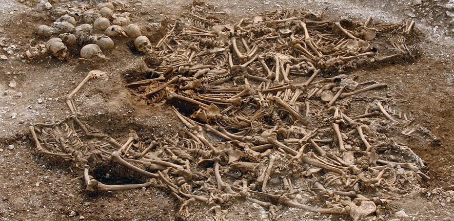
The bones of the Vikings and those they met litter shallow battlefields across the British Isles; two important sites were in Dorset and Oxford. They can be found in the burial sites of Viking groups across the British Isles. And Bones speak.

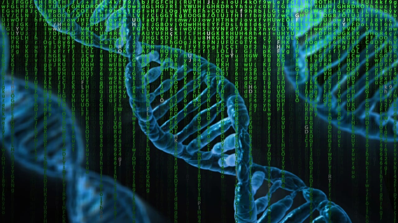
Inside every cell of the human body is DNA; inside blood, inside hair, inside bone. Inside a small bone in the inner ear called the petrous, DNA can sit preserved for tens or even hundreds of thousands of years, if the conditions are right. By sequencing these cells, we can recover the code that tells a human how to be a human.

What ancient Viking DNA tells us about them as specimens

By studying modern humans, it is possible to learn what genes, and mutations to those genes, actually do. This is hard, and very important, but scientists are now building quite a compendium of functions for the human genome. It is one of the key goals of Modern Genomics. It means that we can look at ancient DNA of these Vikings and learn:

Many Vikings actually had brown hair and not blonde hair.
They were evolving to be able to drink milk as adults, like much of Europe
They were evolving to resist certain diseases that may have changed in prevalence.
And much more.

What ancient Viking DNA tells us about them as people

Much better, by studying how these individuals ancestry relates to each other, and modern people, we can learn about who they were, who their parents and grandparents were, what their population was like. This lets us learn:

Early Viking Age raiding parties were an activity for locals and included close family members.
Later Viking Age raiding parties were a much more diverse affair and may have been at a larger scale.
Viking identity was not limited to people with Scandinavian ancestry. These people from Scandinavia received genes from Asia and Southern Europe before the Viking Age.
The genetic legacy in the UK has left the population with up to six per cent Viking DNA.
And perhaps the most interesting finding is that British people could and did become Vikings.

This last finding is really important. The people in the British Isles that were conquered by the Romans were called the “Britons”, and they were culturally Celts, as were the “Picts” or “Painted people” north of Hadrian’s wall where Roman rule ended. Perhaps the last Pictish kingdom was in Orkney and was ended by Viking invasion.

Being captured by Vikings is usually considered a sentence to either death, or slavery. Yet these people integrated into the Viking culture and themselves became Viking – they were buried as Vikings – holding Viking swords and signs of being respected individuals in the local society. Yet some of these people were 100% Pictish by both the mother and fatherline, both in Orkney and Norway. Picts and Scandinavians all became Vikings.

How we know this

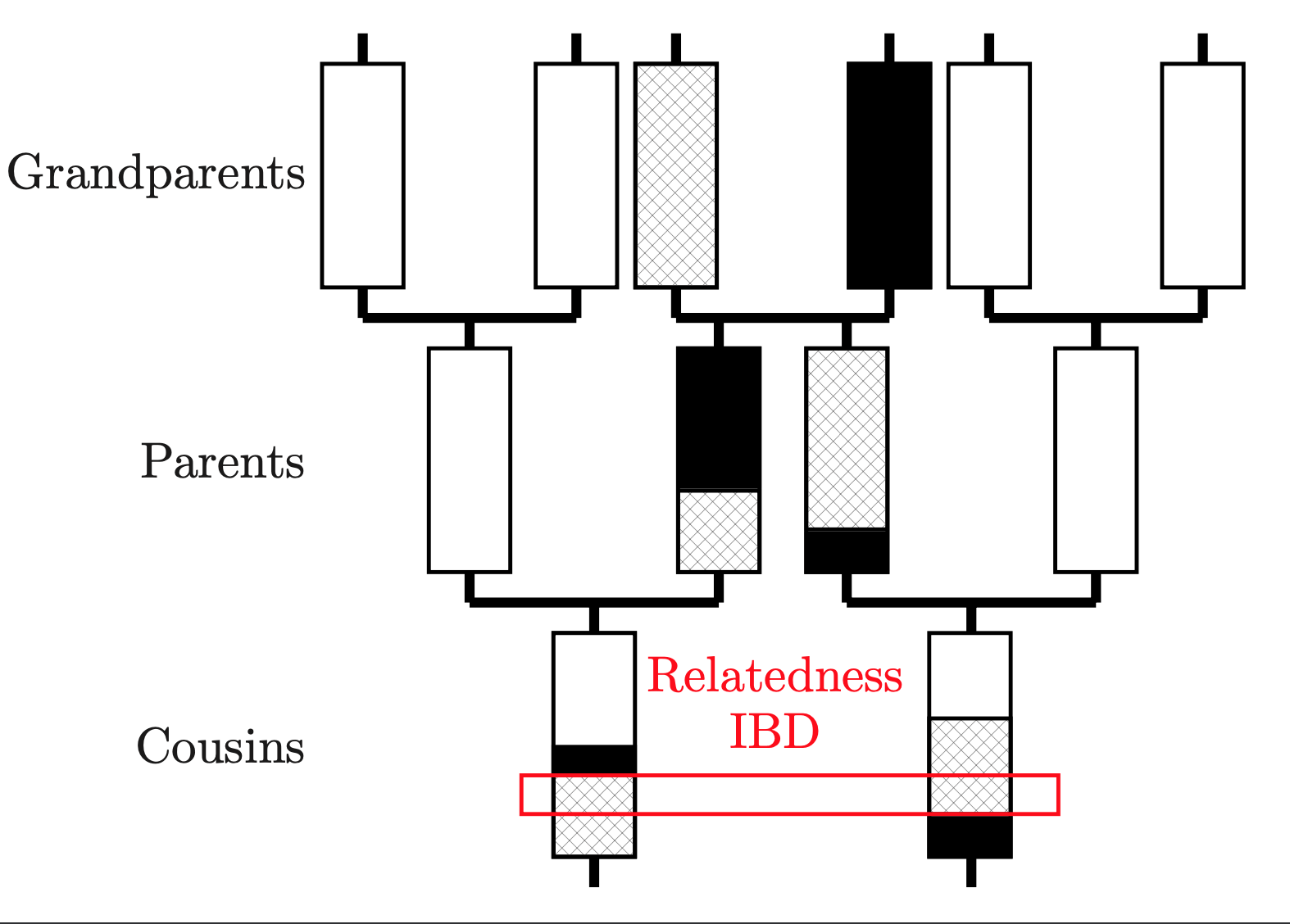
The difference between a Scandinavian and a Pictish genome is, essentially, nothing. These people have the same set of genes. We can still tell who they were though, by examining their genome to ask about who was most related to who. This is possible because genomes are inherited in long chunks that get split approximately in two by a process called recombination every generation. By looking at the length of matches, you can tell how long ago two individuals shared a relative.

How relatedness works for a single strand of DNA (Humans have two). Two cousins share a pair of grandparents, which means that it is likely that they share a segment of ancestry that is the same.

And we can model this. We use a Hidden Markov Model to identify the closest relative for every individual at every position on the genome, which is known as “Chromosome Painting”, because each person is “painted” with everyone else. The maths works like this:

We work through the genome positions $l$ (for $l=1 \ldots L$ ) for a “recipient” individual $i$ who is “painted” with each a reference panel. The painting is over the value of the hidden state $x_{il}=j \in (1 \ldots N, j \ne i)$ f the Hidden Markov model. It describes who is the model’s estimate of the most recent relative.
We compute the probability $Pr(x_{il}=j|x_{i{l-1}}=j^\prime)$ from the transition probabilities. With probability proportional to $e^{d_l} (1-\rho)$ it is the previous state, and with probability proportional to $e^{d_l} \rho$ a “recombination” occurs and it is uniform across all possible states. $d_l$ is the “genetic distance” of genetic marker $l$ and the previous one, called a “recombination map”.
We then match to the data $y_{il}$ which takes values $0$ if the genome does not have a mutation here, and $1$ if it does. We can write $Pr(y_{il}=A|x_{il})= 1-\mu$ if $y_{x_{il}l}=A$ and $\mu$ otherwise. i.e. $\mu$ is the probability of a “mismatch” and we want $\mu$ to be small.
This defines a likelihood which can be handled by the Forward-Backward algorithm, which looks forwards through all the data once and then goes back in the other direction, and due to way the HMM conditioning works this is all that is needed!
We have to learn the parameters $\rho$ and $\mu$ using the Expectation-Maximisation Algorithm.

The way this works is shown in the following cartoon.

Chromosome Painting. We care about the individual at the bottom, who has a particular pattern of mutations (crosses). We use a hidden markov model to identify which individuals are good representatives for a long stretch of DNA, which makes them recent ancestors.

Why do we do this? We know that the true model is not this; it is essentially a giant family tree called the Ancestral Recombination Graph, that changes along the genome due to recombination. This is a beautiful mathematical object but remarkably hard to do inference for! The HMM solution is an example of an embarrassingly parallel algorithm that allows us to get the important information out, without breaking our High Performance Computing facility; we can analyse thousands of individuals at millions of genetic positions this way.

We do this for all individuals. This is quite a lot of data and therefore has to be heavily summarised for modelling; we construct a “similarity matrix” by counting how much genome each pair of individuals shares as the most recent relative. This is chosen because we can write down its distribution and feed it into a clustering algorithm called “FineSTRUCTURE”, which is an implementation of the Stochastic Block Model suitable for genetic data, which uses Reversible Jump Markov-Chain Monte Carlo to learn the populations that are present in a Bayesian framework that accounts for what we know a-priori about how populations should differ. The last thing to do is to describe every individual as a mixture of these populations, which uses Non-negative least squares to learn how much of each individuals’ genome came from which population.

And this leads finally to the estimates of ancestry for each individual: the proportion of their genome from each of the populations we learned.

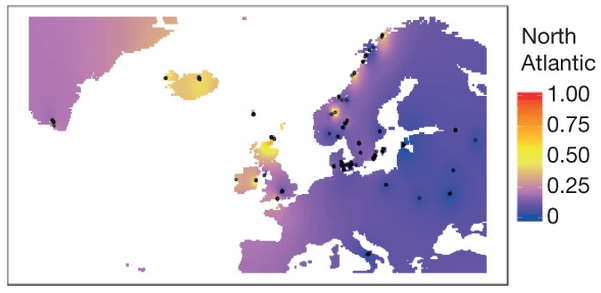
“North Atlantic” ancestry is a careful way of saying “Celtic and Pictish”, i.e. British before the Anglo Saxons. We can plot the density of each ancestry across space using kernel density estimates and we are done. Note the high ancestry estimates of British ancestry in Norway, driven by a couple of individuals with much British ancestry.

Ancient people may not have used data science, but it is a key component in how we understand them today!

There are a lot of moving parts to getting a Data Science algorithm to work in practice. In the analysis above, each step is quite simple, below what a single year in the COMPASS program would teach. Students will get an even deeper understanding of many of these details that are needed for modelling the genetics of Vikings. The key to becoming a good Data Scientist is not in knowing the algorithms – it is knowing how to use them together, and when. That is why an integrated program such as COMPASS is so valuable for training the next generation of Computationally Intensive Statistical Researchers and Data Scientists.