A post by Alexander Modell, PhD student on the Compass programme.

Stein’s paradox in statistics

In 1922, Sir R.A. Fisher laid the foundations of classical statistics with an idea he named maximum likelihood estimation. His principle, for determining the parameters of a statistical model, simply states that given some data, you should choose the parameters which maximise the probability of observing the data that you actually observed. It is based on a solid philosophical foundation which Fisher termed “logic of inductive reasoning” and provides intuitive estimators for all sorts of statistical problems. As a result, it is frequently cited as one of the most influential pieces of applied mathematics of the twentieth century. Eminent statistician Bradley Efron even goes as far as to write

“If Fisher had lived in the era of “apps”, maximum likelihood estimation would have made him a billionaire.” [1]

It came as a major shock to the statistical world when, in 1961, James and Stein exposed a paradox that had the potential to undermine what had become the backbone of classical statistics [2].

It goes something like this.

Suppose I choose a real number on a number line, and instead of telling you that number directly, I add some noise, that is, I perturb it a little and give you that perturbed number instead. We’ll assume that the noise I add is normally distributed and, to keep things simple, has variance one. I ask you to guess what my original number was – what do you do? With no other information to go on, most people would guess the number that I gave them, and they’d be right to do so. By a commonly accepted notion of what “good” is (we’ll describe this a little later on) – this is a “good” guess! Notably, this is also the maximum likelihood estimator.

Suppose now that I have two real numbers and, again, I independently add some noise to each and tell you those numbers. What is your guess of my original numbers? For the same reasons as before, you choose the numbers I gave you. Again, this is a good guess!

Now suppose I have three numbers. As usual, I independently add some noise to each one and tell you those numbers. Of course, you guess the numbers I gave you, right? Well, this no longer the best thing to do! If we imagine those three numbers as a point in three-dimensional space, you can actually do better by arbitrarily choosing some other point, let’s call it B, and shifting your estimate slightly from the point I gave you towards B. This is Stein’s paradox. At first glance, it seems rather absurd. Even after taking some time to take in its simple statement and proof, it’s almost impossible to see how it can possibly be true.

To keep things simple, from now on we will assume that B is the origin, that is that each dimension of B is zero, although keep in mind that all of this holds for any arbitrary point. Stated more formally, the estimator proposed by James and Stein is

$\hat{\mu}_i^{\text{(JS)}} = \left( 1 - \frac{(p-2)}{x_1^2+\cdots + x_p^2} \right) x_i.$

where p is the number of numbers you are estimating, and $x_1,\ldots,x_p$ are the noisy versions that I give you. Since the term in brackets is always less than one, their estimator shrinks each of the dimensions of the observation towards zero. For this reason, it is known as a “shrinkage” estimator. There are two central surprises here. Firstly, it seems totally paradoxical to estimate anything other than the values I gave you. With no other information, why on earth would you estimate anything different? Secondly, their estimate of one value depends on the observations of all of the other values, despite the fact that they’re totally independent!

To most, this is seemingly ludicrous, and to make this point, in his paper on the phenomenon [3], Richard Samworth presents an unusual example. Suppose we want to estimate the proportion of the US electorate who will vote for Barack Obama, the proportion of babies born in China that are girls and the proportion of Britons with light-coloured eyes, then our James-Stein estimate of the proportion of Democratic voters will depend on our hospital and eye colour data!

Before we discuss what we mean when we say that the James-Stein estimator is “better” than the maximum likelihood estimator, let’s take a step back and get some visual intuition as to why this might be true.

Suppose I have a circle on an infinite grid and I task you with guessing the position of the centre of that circle. Instead of just telling you the location of the centre, I draw a point from the circle at random and tell you that position. Let’s call this position A and we’ll call the true, unknown centre of the circle C. What do you propose as your guess? Intuition tells you to guess A, but Stein’s paradox would suggest choosing some other point B, and shifting your guess towards it.

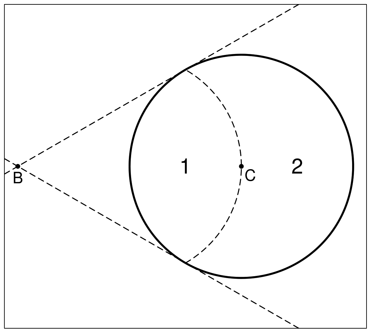Let’s suppose the circle has radius one and its true centre is at $x=0,y=2$ . To keep things simple, suppose I set the point B to be the origin (that is $x=0,y=0$ ). Now, if I randomly draw a point from this circle, what proportion of the time will my guess actually be better if I shrink it slightly towards the point B. For this illustration, we’ll just consider shrinking towards B a very small amount, so we can rephrase this question as this: What proportion of the circle could get closer to the centre if it were shrunk towards B a little?

The answer to that question is the region marked “2” on the figure. A bit of geometry tells us that that’s about 61% of the circle, a little over half. So estimating a point slighter closer to B than the point we drew has the potential to improve our estimate more times than it hinders it! In fact, this holds true regardless of the position of B.

Now let’s consider this problem in three dimensions. We now have a sphere rather than a circle but everything else remains the same. In three dimensions, the region marked “2” covers just over 79% of the sphere, so about four times out of five, our shrinkage estimator does better than estimating the point A. If you’ve just tried to imagine a four-dimensional sphere, your head probably hurts a little but you can still do this maths. Region “2” now covers 87% of the sphere. In ten dimensions, it covers about 98% of the sphere and in one hundred dimensions it covers 99.99999% of it. That is to say, that only one in ten millions times, our estimate couldn’t be improved by shrinking it towards B.

Hopefully, you’re starting it see how powerful this idea can be, and how much more powerful it becomes as we move into higher dimensions. Despite this, the more you think about it, the more something seems amiss – yet it’s not.

Statisticians typically determine how “good” an estimator is through what is called a loss function. A loss function can be viewed as a penalty that increases the further your estimate is from the underlying truth. Examples are the squared error loss $\ell_2(\hat{\mu};\mu) = \sum_i(\hat{\mu}_i - \mu_i)^2,$ which is by far the most common choice, and the absolute error loss $\ell_1(\hat{\mu};\mu)\ = \sum_i |\hat{\mu}_i - \mu_i|$ where $\hat{\mu}$ is the estimate and $\mu$ is the truth. Since the loss function depends on the data that was observed, it is not suitable for comparing estimators, so instead the risk of the estimator is used, which is defined as the loss we would expect to see if we drew a random dataset from the underlying distribution.

The astonishing result that James and Stein proved, was that, under the squared error loss, their “shrinkage” estimator has a lower risk than the maximum likelihood estimator, regardless of the underlying truth. This came as a huge surprise to the statistics community at the time, which was firmly rooted in Fisher’s principle of maximum likelihood estimation.

It is natural to ask whether this is a quirk of the normal distribution and the squared error loss, but in fact, similar phenomena have been shown for a wide range of distributions and loss functions.

It would be easy to shrug this result off as merely a mathematical curiosity – many contemporaries of Stein did – yet in the era of big data, the ideas underpinning it have proved crucial to modern statistical methodology. Modern datasets regularly contain tens of thousands, if not millions of dimensions and in these settings, classical statistical ideas break down. Many modern machine learning algorithms, such as ridge and Lasso regression, are underpinned by these ideas of shrinkage.

References

[1]: Efron, B., & Hastie, T. (2016). Computer age statistical inference (Vol. 5). Cambridge University Press.

[2]: James, W. and Stein, C.M. (1961) Estimation with Quadratic Loss. Proceedings of the Fourth Berkeley Symposium on Mathematical Statistics and Probability, 1, 361-379, University California Press, Berkeley.

[3]: Samworth, R. J., & Cambridge, S. (2012). Stein’s paradox. eureka, 62, 38-41.