Student Perspectives: Change in the air: Tackling Bristol’s nitrogen oxide problem

A post by Dom Owens, PhD student on the Compass programme.

“Air pollution kills an estimated seven million people worldwide every year” – World Health Organisation

Many particulates and chemicals are present in the air in urban areas like Bristol, and this poses a serious risk to our respiratory health. It is difficult to model how these concentrations behave over time due to the complex physical, environmental, and economic factors they depend on, but identifying if and when abrupt changes occur is crucial for designing and evaluating public policy measures, as outlined in the local Air Quality Annual Status Report. Using a novel change point detection procedure to account for dependence in time and space, we provide an interpretable model for nitrogen oxide (NOx) levels in Bristol, telling us when these structural changes occur and describing the dynamics driving them in between.

Model and Change Point Detection

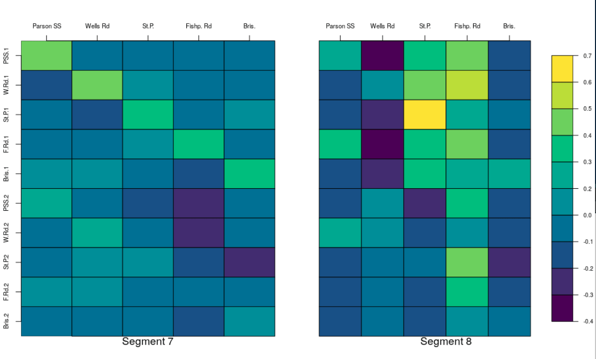
We model the data with a piecewise-stationary vector autoregression (VAR) model:

In between change points the time series $\boldsymbol{Y}_{t}$ , a $d$ -dimensional vector, depends on itself linearly over $p \geq 1$ previous time steps through parameter matrices $\boldsymbol{A}_i^{(j)}, i=1, \dots, p$ with intercepts $\boldsymbol{\mu}^{(j)}$ , but at unknown change points $k_j, j = 1, \dots, q$ the parameters switch abruptly. $\{ \boldsymbol{\varepsilon}_{t} \in \mathbb{R}^d : t \geq 1 \}$ are white noise errors, and we have $n$ observations.

We phrase change point detection as a test of the hypotheses $H_0: q = 0$ vs. $H_1: q \geq 1$ , i.e. the null states there is no change, and the alternative supposes there are possibly multiple changes. To test this, we use moving sum (MOSUM) statistics $T_k(G)$ extracted from the model; these compare the scaled difference between prediction errors for $G$ steps before and after $k$ ; when $k$ is in a stationary region, $T_k(G)$ will be close to zero, but when $k$ is near or at a change point, $T_k(G)$ will be large. If the maximum of these exceeds a threshold suggested by the distribution under the null, we reject $H_0$ and estimate change point locations with local peaks of $T_k(G)$ .

Air Quality Data

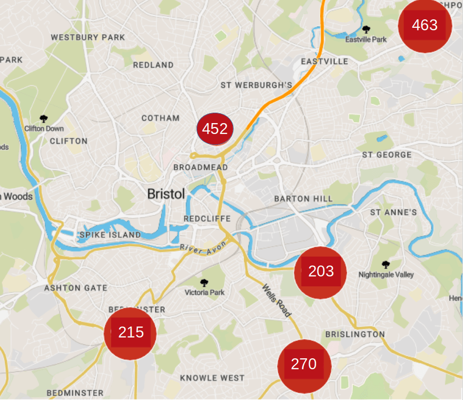
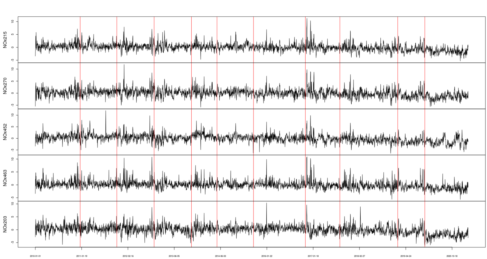
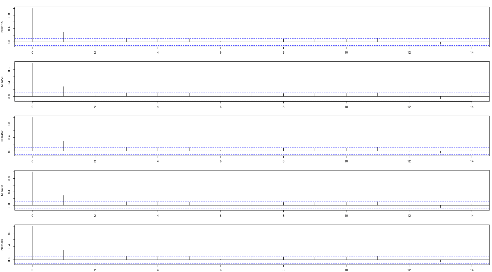
With data from Open Data Bristol over the period from January 2010 to March 2021, we have hourly readings of NOx levels at five locations (with Site IDs) around the city of Bristol, UK: AURN St Paul’s (452); Brislington Depot (203); Parson Street School (215); Wells Road (270); Fishponds Road (463). Taking daily averages, we control for meteorological and seasonal effects such as temperature, wind speed and direction, and the day of the week, with linear regression then analyse the residuals.

Residual series with estimated change points in red

We use the bandwidth $G=280$ days to ensure estimation accuracy relative to the number of parameters, which effectively asserts that two changes cannot occur in a shorter time span. The MOSUM procedure rejects the null hypothesis and detects ten changes, pictured above. We might attribute the first few to the Joint Local Transport Plan which began in 2011, while the later changes may be due to policy implemented after a Council supported motion in November 2016. The image below visualises the estimated parameters around the change point in November 2016; we can see that in the segment seven there is only mild cross-dependence, but in segment eight the readings at Wells Road, St. Paul’s, and Fishponds Road become strongly dependent on the other series.

Estimated parameters for segments seven and eight, with lagged variables by row

ACF of entire series at site 215 over three time scales

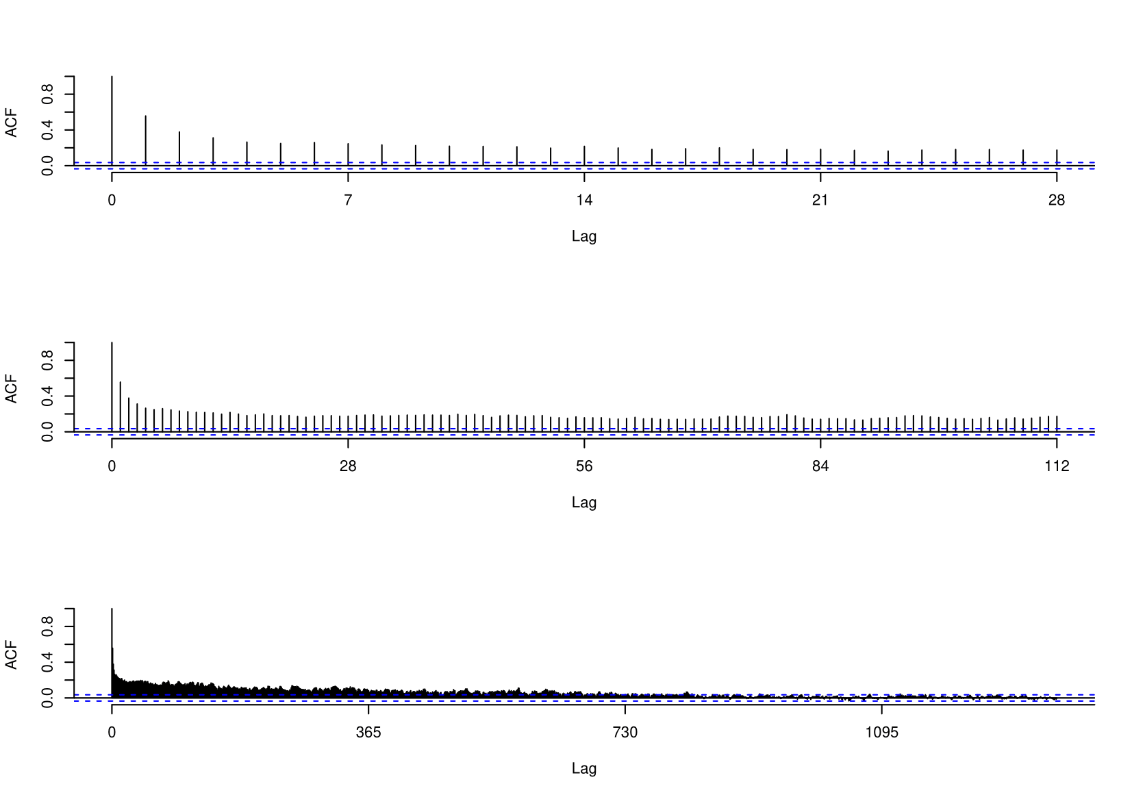
Scientists have generally worked under the belief that these concentration series have long-memory behaviour, meaning values long in the past have influence on today’s values, and that this explains why the autocorrelation function (ACF) decays slowly, as seen above. Perhaps the most interesting conclusion we can draw from this analysis is that that structural changes explain this slow decay – the image below displays much shorter range dependence for one such stationary segment.

Conclusion

After all our work, we have a simple, interpretable model for NOx levels. In reality, physical processes often depend on each other in a non-linear fashion, and according to the geographical distances between where they are measured; accounting for this might provide better predictions, or tell a slightly different story. Moreover, there should be interactions with the other pollutants present in the air. Could we combine these for a large-scale, comprehensive air quality model? Perhaps the most important question to ask, however, is how this analysis can be used to benefit policy makers. If we could combine this with a causal model, we might we be able to identify policy outcomes, or to draw comparisons with other regions.