Introduction

My work focuses on addressing the growing need for reliable, day-ahead energy demand forecasts in smart grids. In particular, we have been developing structured ensemble models for probabilistic forecasting that are able to incorporate information from a number of sources. I have undertaken this EDF-sponsored project with the help of my supervisors Matteo Fasiolo (UoB) and Yannig Goude (EDF) and in collaboration Christian Capezza (University of Naples Federico II).

Motivation

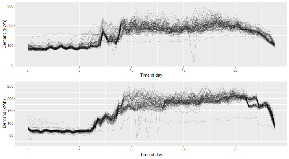
One of the largest challenges society faces is climate change. Decarbonisation will lead to both a considerable increase in demand for electricity and a change in the way it is produced. Reliable demand forecasts will play a key role in enabling this transition. Historically, electricity has been produced by large, centralised power plants. This allows production to be relatively easily tailored to demand with little need for large-scale storage infrastructure. However, renewable methods are typically decentralised, less flexible and supply is subject to weather conditions or other unpredictable factors. A consequence of this is that electricity production will less able to react to sudden changes in demand, instead it will need to be generated in advance and stored. To limit the need for large-scale and expensive electricity storage and transportation infrastructure, smart grid management systems can instead be employed. This will involve, for example, smaller, more localised energy storage options. This increases the reliance on accurate demand forecasts to inform storage management decisions, not only at the aggregate level, but possibly down at the individual household level. The recent impact of the Covid-19 pandemic also highlighted problems in current forecasting methods which struggled to cope with the sudden change in demand patterns. These issues call attention to the need to develop a framework for more flexible energy forecasting models that are accurate at the household level. At this level, demand is characterised by a low signal-to-noise ratio, with frequent abrupt changepoints in demand dynamics. This can be seen in Figure 1 below.

Figure 1: Demand profiles for two different customers. Portuguese smart meter data [4].

The challenges posed by forecasting at a low level of aggregation motivate the use of an ensemble approach that can incorporates information from several models and across households. In particular, we propose an additive stacking structure where we can borrow information across households by constructing a weighted combination of experts, which is generally referred to as stacking regressions [2].

Additive stacking

Additive stacking is a probabilistic ensemble method where we form a weighted mixture distribution of multiple predictive densities. We begin by dividing our data into 3 parts.

Expert training: The data we use to train the component models of the ensemble
Stacking: The data we use to fit the weights
Validation set: The data we use to evaluate the performance of our ensemble.

We first fit our experts (individual models) using the expert training data. We then find the predictive densities of our fitted experts on the stacking data. Suppose in our stacking data we have data points $(\mathbf{X}_{i}, y_{i})$ for $i \in \{1,\dots, N\}$ and fitted predictive densities $p_{k}(\mathbf{X}_{i}, y_{i})$ for $k \in \{1,\dots,K\}$ . For ease of notation we will let $p_{k}(\mathbf{X}_{i}, y_{i}) = p_{ki}$ . Then our stacked model has the general likelihood:

$\mathcal{L}(\boldsymbol{\alpha}|\mathbf{p}) = \prod_{i=1}^{N}\left(\sum_{k=1}^{K} \alpha_{ki} p_{ki} \right).$

Where $\alpha_{ki}$ are the weights. We want to find the weights that maximse this likelihood with respect to the constraints:

$\sum_{k=1}^{K}\alpha_{ki} = 1.$
$\alpha_{ki} > 0.$

We want the weights to depend on some features from our data. This idea was explored by Capezza using multinomial weights of the form:

$\alpha_{ki} = \frac{\exp(\eta_{ki})}{\sum_{\alpha=1}^{K}\exp(\eta_{\alpha i})}.$

Where $\eta_{ki}$ is determined by some set of features. We do not only include linear combinations of features but also, random or smooth effects based on spline basis expansions. These can be fitted using the methods in Wood et al (2016). A key limitation of the multinomial weights is that there is a huge amount of flexibility as each weight has it’s own $\eta$ which can lead to overfitting. Another problem is that the number of unknown parameters required to estimate grows linearly with the number of experts. This limits the number of experts and thus the amount of information that can be given to the model as it becomes too computationally complex to fit. This motivated the idea of more structured weights that, at the cost of flexibility, would be less prone to overfitting and more efficient to compute.

Ordinal weights

In order to reduce the number of unknown parameters, we first need to make an assumption about the experts. In this case we assume that the experts have some associated ordering. For example, we could use a set of experts that looked at the previous day, week and month and order them accordingly. We treat the experts as though they are responses in an ordinal regression and use the framework of Winship and Mare (1984) to parametrise the weights. This involves fitting a set of thresholds $[\theta_{1}, \theta_{2},\dots,\theta_{K-1}]$ such that $\theta_{i} > \theta_{i-1} \forall i$ . We can ensure this property holds by parameterising the thresholds as $\theta_{1} = \tau_{1}$ and,

$\theta_{k} = \tau_{1} + \sum_{i=2}^{k}\exp(\tau_{i}) \forall k \in \{2,\dots,K-1\}.$

The weight of expert $k$ at point $i$ is then,

$\alpha_{ki} = F(\theta_{k} - \eta_{i}) - F(\theta_{k-1} - \eta_{i}).$

Where $F(\cdot)$ can be any cumulative distribution function, but as a standard we use the logit function,

$F(x) = \frac{\exp(x)}{1+\exp(x)}.$

The weights of the experts at each data point are now entirely determined by a single $\eta$ and the cut points. To see how the weights change with $\eta$ you can use the interactive plot below. The area under the curve for each of the colours corresponds to the weighting. The cutpoints are represented by the vertical lines.

Future work

A limitation of the ordered structure is that it relies on an assumption about the experts. That is, that they must have some associated order. This significantly restricts the number of available experts that you can use. The next step is to create a framework that allows an ordinal weighting structure to be used in conjunction with unordered experts as well. Thus we would retain the modelling advantages of the ordered framework with the flexibility of a multinomial structure.

References

[1] Christian Capezza, Biagio Palumbo, Yannig Goude, Simon N. Wood, and Matteo Fasiolo. Additive stacking for disaggregate electricity demand forecasting, 2020.

[2] David H. Wolpert. Stacked generalization. Neural Networks, 5(2):241–259, 1992a. ISSN 0893-6080. doi: https://doi.org/10.1016/S0893-6080(05)80023-1.

[3] Simon N. Wood, Natalya Pya, and Benjamin S ̈afken. Smoothing parameter and model selection for general smooth models. Journal of the American Statistical Association, 111(516):1548–1563, 2016. doi: 10.1080/01621459.2016.1180986.

[4] Trindade (2015), Electricity Load Diagrams, Retrieved from: https://archive.ics.uci.edu/ml/datasets/ElectricityLoadDiagrams20112014