
A post by Dan Ward, PhD student on the Compass programme.
Normalising flows are black-box approximators of continuous probability distributions, that can facilitate both efficient density evaluation and sampling. They function by learning a bijective transformation that maps between a complex target distribution and a simple distribution with matching dimension, such as a standard multivariate Gaussian distribution.
Transforming distributions
Before introducing normalising flows, it is useful to introduce the idea of transforming distributions more generally. Lets say we have two uniform random variables, ")
")

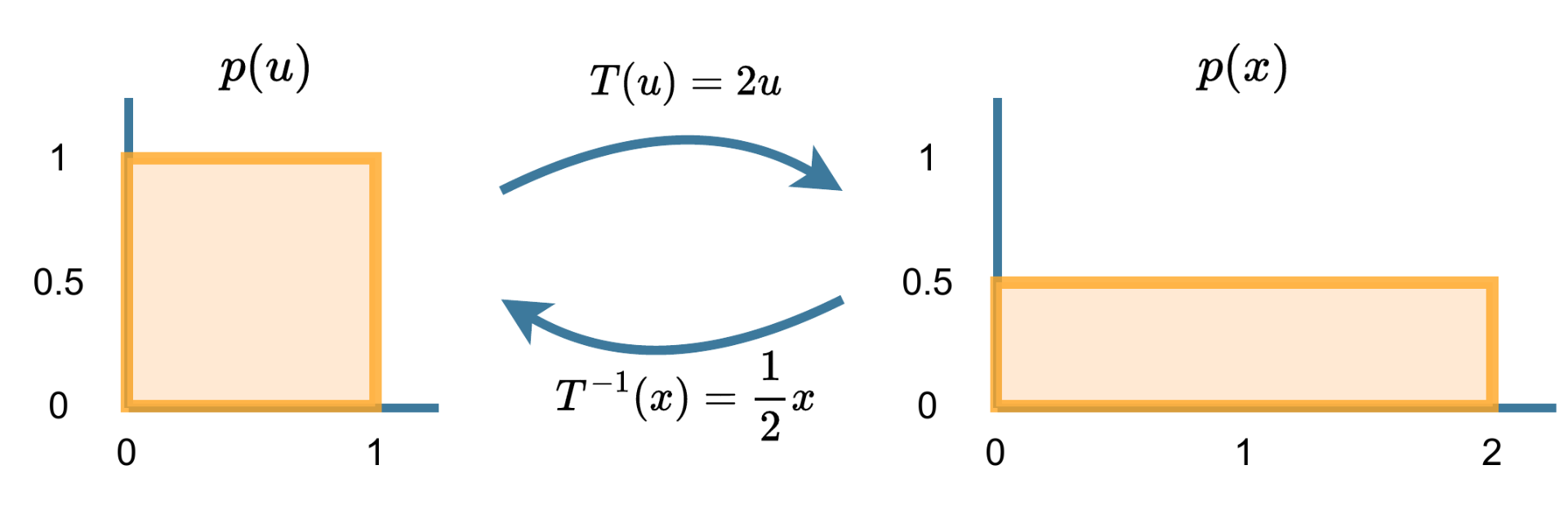
If we wished to sample ")
")
")
= p(u=T^{-1}(x)) \cdot 2^{-1},")
where )")

")
This idea can be made more precise and be generalised to the multivariate case, using the change of variables formula
 = p(u=T^{-1}(x))\vert \text{det}\ J_T(u) \vert^{-1}, \quad (1)")
where ")
")
 = \begin{pmatrix} \frac{\partial x_1}{\partial u_1} & \cdots & \frac{\partial x_1}{\partial u_D} \\ \vdots & \ddots & \vdots \\ \frac{\partial x_D}{\partial u_1} & \cdots & \frac{\partial x_D}{\partial u_D} \\ \end{pmatrix}.")
The absolute value of the Jacobian determinant,  \vert")

 \vert > 1")
 < p(u)")
 \vert < 1")
 > p(u)")

 = p(u=T^{-1}(x)) \vert \text{det}\ J_{T^{-1}}(x) \vert, \quad (2)")
Normalising flows
Normalising flows are a simple extension of the above, in which we approximate a target distribution ")


")
")
Note that it is also straight forward to learn conditional distributions, by making the bijection
Choice of transformation
Much of recent normalising flow research has focused on the choice of
- Flexibility. The transformation should be flexible enough to be able to mould the base distribution into the target density. One simple way to increase flexibility is to compose multiple bijections, i.e.
.
- Fast
and
computation. For density evaluation to be fast, both
must be fast to compute. Generally,
is constrained to be triangular, in which case the determinant can be efficiently computed as the product of the diagonal entries.
- Fast
In practice, there is often a trade off between these components that should be considered for the task at hand. There are a diverse range of choices for
For training we need some “information” about the target density, typically either samples from the target distribution, or the ability to evaluate the target density (potentially up to a normalising constant). We consider how to train a flow in these contexts in the next section.
Training
Using Samples. Training a flow using samples ")
,")
![\approx - \frac{1}{N} \sum_{i=1}^N \left[ \log p(u=T_\phi^{-1}(x_i)) + \log \big\vert \text{det}\ J_{T_\phi^{-1}}(x_i) \big\vert \right],](https://s0.wp.com/latex.php?latex=%5Capprox+-+%5Cfrac%7B1%7D%7BN%7D+%5Csum_%7Bi%3D1%7D%5EN+%5Cleft%5B+%5Clog+p%28u%3DT_%5Cphi%5E%7B-1%7D%28x_i%29%29+%2B+%5Clog+%5Cbig%5Cvert+%5Ctext%7Bdet%7D%5C+J_%7BT_%5Cphi%5E%7B-1%7D%7D%28x_i%29+%5Cbig%5Cvert+%5Cright%5D%2C&bg=ffffff&fg=000000&s=0 "\approx - \frac{1}{N} \sum_{i=1}^N \left[ \log p(u=T_\phi^{-1}(x_i)) + \log \big\vert \text{det}\ J_{T_\phi^{-1}}(x_i) \big\vert \right],")
where in the second line we substitute in equation 2. Note that this can equivalently be framed as minimising the “forward” Kullback-Leibler (KL) divergence between the true and approximate distributions as
![D_{KL} \left[p^*(x)||p_\phi(x)\right] = \mathbb{E}_{p^*(x)}\left[\log p^*(x) - \log p_\phi(x) \right],](https://s0.wp.com/latex.php?latex=D_%7BKL%7D+%5Cleft%5Bp%5E%2A%28x%29%7C%7Cp_%5Cphi%28x%29%5Cright%5D+%3D+%5Cmathbb%7BE%7D_%7Bp%5E%2A%28x%29%7D%5Cleft%5B%5Clog+p%5E%2A%28x%29+-+%5Clog+p_%5Cphi%28x%29+%5Cright%5D%2C&bg=ffffff&fg=000000&s=0 "D_{KL} \left[p^*(x)||p_\phi(x)\right] = \mathbb{E}_{p^*(x)}\left[\log p^*(x) - \log p_\phi(x) \right],")
![= - \mathbb{E}_{p^*(x)}[\log p_\phi(x)] + \text{const.}](https://s0.wp.com/latex.php?latex=%3D+-+%5Cmathbb%7BE%7D_%7Bp%5E%2A%28x%29%7D%5B%5Clog+p_%5Cphi%28x%29%5D+%2B+%5Ctext%7Bconst.%7D&bg=ffffff&fg=000000&s=0 "= - \mathbb{E}_{p^*(x)}[\log p_\phi(x)] + \text{const.}")
The ability to fit flows by maximum likelihood is generally seen as a key advantage of normalising flows, making them simpler to train than other generative models such as generative adversarial networks.
Using density evaluations. In many areas of statistics, we can often only evaluate the density of a target distribution up to a normalising constant 
 = \frac{\tilde{p}(x)}{C}")
")
![D_{KL}\left[p_\phi(x) \vert \vert p^*(x)\right] = \mathbb{E}_{p_\phi(x)} \left[\log p_\phi(x) - \log p^*(x) \right],](https://s0.wp.com/latex.php?latex=D_%7BKL%7D%5Cleft%5Bp_%5Cphi%28x%29+%5Cvert+%5Cvert+p%5E%2A%28x%29%5Cright%5D+%3D+%5Cmathbb%7BE%7D_%7Bp_%5Cphi%28x%29%7D+%5Cleft%5B%5Clog+p_%5Cphi%28x%29+-+%5Clog+p%5E%2A%28x%29+%5Cright%5D%2C&bg=ffffff&fg=000000&s=0 "D_{KL}\left[p_\phi(x) \vert \vert p^*(x)\right] = \mathbb{E}_{p_\phi(x)} \left[\log p_\phi(x) - \log p^*(x) \right],")
![= \mathbb{E}_{p(u)} \left[ \log p(u) - \log \vert \text{det} J_{T_\phi}(u) \vert -\log p^*(x=T_\phi(u)) \right],](https://s0.wp.com/latex.php?latex=%3D+%5Cmathbb%7BE%7D_%7Bp%28u%29%7D+%5Cleft%5B+%5Clog+p%28u%29+-+%5Clog+%5Cvert+%5Ctext%7Bdet%7D+J_%7BT_%5Cphi%7D%28u%29+%5Cvert+-%5Clog+p%5E%2A%28x%3DT_%5Cphi%28u%29%29+%5Cright%5D%2C+&bg=ffffff&fg=000000&s=0 "= \mathbb{E}_{p(u)} \left[ \log p(u) - \log \vert \text{det} J_{T_\phi}(u) \vert -\log p^*(x=T_\phi(u)) \right],")
![= \mathbb{E}_{p(u)} \left[ - \log \vert \text{det} J_{T_\phi}(u) \vert -\log \tilde{p}(x=T_\phi(u)) \right] + \text{const.}](https://s0.wp.com/latex.php?latex=%3D+%5Cmathbb%7BE%7D_%7Bp%28u%29%7D+%5Cleft%5B+-+%5Clog+%5Cvert+%5Ctext%7Bdet%7D+J_%7BT_%5Cphi%7D%28u%29+%5Cvert+-%5Clog+%5Ctilde%7Bp%7D%28x%3DT_%5Cphi%28u%29%29+%5Cright%5D+%2B+%5Ctext%7Bconst.%7D&bg=ffffff&fg=000000&s=0 "= \mathbb{E}_{p(u)} \left[ - \log \vert \text{det} J_{T_\phi}(u) \vert -\log \tilde{p}(x=T_\phi(u)) \right] + \text{const.}")
![\approx -\frac{1}{N} \sum_{i=1}^N \left[ \log \tilde{p}(x=T_\phi(u_i)) + \log \vert \text{det}\ J_{T_\phi}(u_i) \vert \right] + \text{const}.](https://s0.wp.com/latex.php?latex=%5Capprox+-%5Cfrac%7B1%7D%7BN%7D+%5Csum_%7Bi%3D1%7D%5EN+%5Cleft%5B+%5Clog+%5Ctilde%7Bp%7D%28x%3DT_%5Cphi%28u_i%29%29+%2B+%5Clog+%5Cvert+%5Ctext%7Bdet%7D%5C+J_%7BT_%5Cphi%7D%28u_i%29+%5Cvert+%5Cright%5D+%2B+%5Ctext%7Bconst%7D.&bg=ffffff&fg=000000&s=0 "\approx -\frac{1}{N} \sum_{i=1}^N \left[ \log \tilde{p}(x=T_\phi(u_i)) + \log \vert \text{det}\ J_{T_\phi}(u_i) \vert \right] + \text{const}.")
where we make use of ")
Flows in practice – flowjax
There are now many available packages that make it straight forward to use normalising flows. Here, I will show how normalising flows can be used in Python, using the flowjax Python package. It’s a great package with very easy to use Jax-based implementations of flows (disclaimer: I may be biased as the author of this package – other normalising flow packages are available, such as the PyTorch-based nflows).
First we need to import the required packages
from flowjax.distributions import Normal
from flowjax.flows import BlockNeuralAutoregressiveFlow
from flowjax.train_utils import train_flow
from jax import random
import jax.numpy as jnp
import import numpy as np
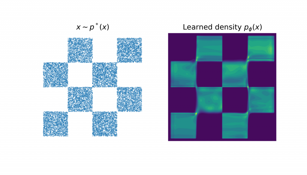
We can create some toy data, which are points following a chequered pattern
def get_chequered_data(n=100000):
x1 = np.random.rand(n) * 4 - 2
x2 = np.random.rand(n) - np.random.randint(0, 2, n) * 2
x2 = x2 + (np.floor(x1) % 2)
return jnp.column_stack((x1, x2))*2
x = get_chequered_data()
We can now create and train the flow. Here we use a block neural autoregressive flow model, as introduced by De Cao et al. [2020].
flowkey, trainkey = random.split(random.PRNGKey(1)) # Jax random seeds
base_dist = Normal(x.shape[1])
flow = BlockNeuralAutoregressiveFlow(flowkey, base_dist, block_size=(50, 50), nn_layers=3)
flow, _ = train_flow(trainkey, flow, x, learning_rate=1e-2, max_epochs=150, max_patience=20)
After training, we can evaluate the density of arbitrary points flow.log_prob(x[:10]), or sample (if flow.sample(key, n=10).Visualising the learned density, we can see the flow reasonably approximates the target density
The learned density
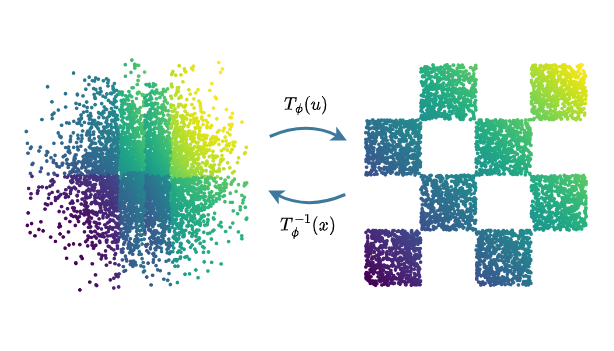
We can also visualise the learned transformation. Note the colours below are to give an indication of which points map to which between the two distributions.
The learned transformation
If you are interested in learning more about normalising flows, I would recommend this review paper by Papamakarios et al. [2020], for a more complete, but still introductory overview.
References
De Cao, N., Aziz, W. and Titov, I., 2020, August. Block neural autoregressive flow. In Uncertainty in artificial intelligence (pp. 1263-1273). PMLR.
Papamakarios, G., Nalisnick, E.T., Rezende, D.J., Mohamed, S. and Lakshminarayanan, B., 2021. Normalizing Flows for Probabilistic Modeling and Inference. J. Mach. Learn. Res., 22(57), pp.1-64.