A post by Annie Gray, PhD student on the Compass programme.

Introduction

Initially, my Compass mini-project aimed to explore what we can discover about objects given a matrix of similarities between them. More specifically, how to appropriately measure the distance between objects if we represent each as a point in $\mathbb{R}^p$ (the embedding), and what this can tell us about the objects themselves. This led to discovering that the geodesic distances in the embedding relate to the Euclidean distance between the original positions of the objects, meaning we can recover the original positions of the objects. This work has applications in fields that work with relational data for example: genetics, Natural Language Processing and cyber-security.

This work resulted in a paper [3] written with my supervisors (Nick Whiteley and Patrick Rubin-Delanchy), which has been accepted at NeurIPS this year. The following gives an overview of the paper and how the ideas can be used in practice.

Matrix factorisation and the interpretation of geodesic distance

Given a matrix of relational information such as a similarity, adjacency or covariance matrix, we consider the problem of finding the distance between objects and so their true positions. For now, we focus on the case when we have an undirected graph of $n$ objects with associated adjacency matrix, that is,

$A_{ij} = \Bigg\{ \begin{array}{ll} 1 & \text{ if nodes } i \text{ and } j \text{ are connected}\\ 0, & \text{ otherwise}.\end{array}$

Further, we assume that this graph follows a latent position model which means our adjacency matrix has the form,

$A_{ij} \overset{ind}{\sim} \text{Bernoulli}\{P_{ij}\} \text{ for } i<j,$

where the probability that two nodes are connected $P_{ij} = f(Z_i,Z_j)$ is given by some real-valued symmetric function $f$ called the kernel which relate to unobserved vectors $Z_1,\ldots,Z_n \in \mathbb{R}^d$ , as shown in Figure 1. In our setup we assume that $f$ will be nonnegative definite Mercer kernel, meaning $f$ can be written as the inner-product of the associated Mercer feature $\phi$ : $f(Z_i,Z_j) = \langle \phi (Z_i),\phi (Z_j) \rangle$ .

**Figure 1:** Formation of the adjacency matrix from a graph and probability matrix.

Broadly stated, our goal is to recover $Z_1, \ldots, Z_n$ given $A$ , up to identifiability constraints. We seek a method to perform this recovery that can be implemented in practice without any knowledge of $f$ , nor of any explicit statistical model for $A$ , and to which we can plug in various matrix-types, be it adjacency, similarity, covariance, or other. At face value, this seems a lot to ask, however, under quite general assumptions, we show that a practical solution is provided by the key combination of two procedures:

matrix factorisation of $A$ , such as spectral embedding,
followed by nonlinear dimension reduction, such as Isomap [2].

This combination of techniques is often used in applications, however, often with little rigorous justification. Here we show why tools that approximate and preserve geodesic distance work so well.

Step 1: Spectral embedding

Graph embedding is a common first step when performing statistical inference on networks as it seeks to represent each node as a point while preserving relationships between nodes. Spectral embedding can be interpreted as seeking to position nodes in such a way that a node sitting between nodes $x$ and $y$ acts as the corresponding probabilistic mixture of the two.

For $p \leq n$ , we define the $p$ -dimensional spectral embedding of $A$ to be $\hat{X}=[\hat X_1, \ldots, \hat X_n]^\top= \hat{U} |\hat{S}|^{1/2} \in \mathbb{R}^{n \times p}$ , where $|\hat{S}| \in \mathbb{R}^{p \times p}$ is a diagonal matrix containing the absolute values of the $p$ largest eigenvalues of $A$ , by magnitude, and $\hat{U }\in \mathbb{R}^{n \times p}$ is a matrix containing corresponding orthonormal eigenvectors, in the same order. Because of the nonnegative definite assumption on $f$ , we have $A\approx \hat{X}\hat{X}^T$ for large enough $p$ , under reasonable assumptions (illustrated in Figure 2). One should think of $\hat X_i$ as approximating the vector of first $p$ components of $X_i = \phi(Z_i)$ , up to orthogonal transformation, and this can be formalised to a greater or lesser extent depending on what assumptions are made.

**Figure 2:** Illustration of theory. We find a precise relationship between the geodesic distance, and the Euclidean distance, in latent space.

Step 2: Isomap

It is known that the high-dimensional images $X_i = \phi(Z_i)$ , live near a low-dimensional manifold [1]. The spectral embedding step approximates high-dimensional images of the $Z_i$ ‘s, living near a $d$ -dimensional manifold (shown in Figure 2). Our paper shows that the distance between the $Z_i$ ‘s is encoded in these high-dimensional images as the ‘distance along the manifold’, called the geodesic distance. Under general assumptions, geodesic distance in this manifold equals Euclidean distance in latent space, up to simple transformations of the coordinates, for example scaling. Pairwise geodesics distances can be estimated using a nonlinear dimension reduction and from this estimates for the latent positions can be found.

The nonlinear dimension reduction tool we focus on is Isomap as it computes a low-dimensional embedding based on the geodesic distances:

Input: $p$ -dimensional points $\hat X_1, \ldots, \hat X_n$
Compute the neighbourhood graph of radius $\epsilon$ : a weighted graph connecting $i$ and $j$ , with weight $\|\hat X_i - \hat X_j\|$ , if $\|\hat X_i - \hat X_j\| \leq \epsilon$
Compute the matrix of shortest paths on the neighbourhood graph, $\hat{D}_{\mathcal{M}} \in \mathbb{R}^{n \times n}$
Apply classical multidimensional scaling (CMDS) to $\hat{D}_{\mathcal{M}}$ into $\mathbb{R}^d$
Output: $d$ -dimensional points $\hat Z_1, \ldots, \hat Z_n$

Simulated data example

**Figure 3:** True latent positions for subgrid of 100 points.

This section shows the theory at work in a pedagogical example using simulated data of points on a grid. To show the improvement of latent position recovery as the number of nodes increases, we make the grid finer, with $n = 100, 400, 1600, 6400$ . To aid visualisation, all plots of latent positions shown are a subset of $100$ estimated positions corresponding to true positions on a sub-grid which are common across $n$ and are coloured according to their true $y$ -coordinate as shown in Figure 3.

Consider an undirected random graph following a latent position model with kernel

$f(x,y) = \{\cos(x^{(1)} - y^{(1)}) + \cos(x^{(2)} - y^{(2)}) +2\}/4$ . In this paper, we show that for kernels which are translation invariant, meaning they are of the form $f(x,y) = g(x-y)$ , the geodesic distances between $X_i$ and $X_j$ are equal to the Euclidean distances between $Z_i$ and $Z_j$ , up to linear transformation.

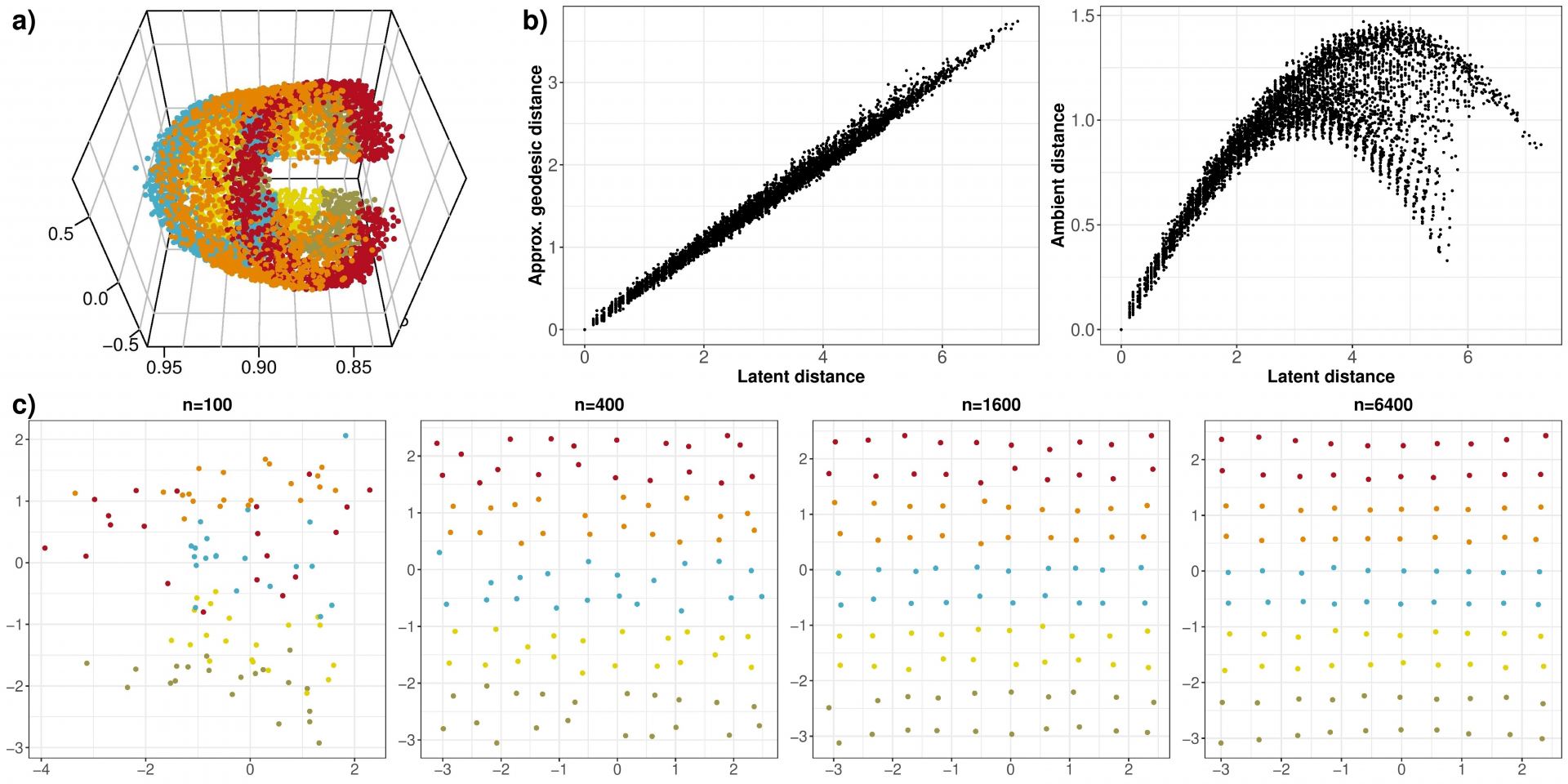
For each $n = 100, 400, 1600, 6400$ , we simulate a graph, and its spectral embedding $\hat X_1, \ldots, \hat X_n$ into $p=5$ dimensions. The first three dimensions of this embedding are shown in Figure 4a), and we see that the points gather about a two-dimensional, curved, manifold. Whilst looking at this figure, it is not obvious that we would have a linear relationship between the geodesic distances and the Euclidean distances in latent space, however, 4b) shows this is true up to scaling, whereas there is significant distortion between ambient and latent distance ( $\lVert \hat X_i - \hat X_j \rVert$ versus $\lVert Z_i - Z_j \rVert$ ). Finally, we recover the estimated latent positions in $\mathbb{R}^2$ using Isomap, in Figure 4c). As the theory predicts, the recovery error vanishes as $n$ increases.

**Figure 4:** a) Spectral embedding (first 3 dimensions), b) comparison of latent, approximate geodesic, and ambient distance and c) latent position recovery in the dense regime by spectral embedding followed by Isomap for increasing n.

Additionally in the paper, we look at when the graph is sparse, and the recovery error still shrinks, but more slowly. We also implement other related approaches: UMAP, t-SNE applied to spectral embedding, node2vec directly into two dimensions and node2vec in ten dimensions followed by Isomap. Together, these results support the central recommendation: to use matrix factorisation (e.g. spectral embedding, node2vec), followed by nonlinear dimension reduction (e.g. Isomap, UMAP, t-SNE).

Conclusion

Our research shows how matrix-factorisation and dimension-reduction can work together to reveal the true positions of objects based only on pairwise similarities such as connections or correlations.

References

[1] Rubin-Delanchy, Patrick. “Manifold structure in graph embeddings.” Advances in Neural Information Processing Systems 33 (2020).

[2] Tenenbaum, Joshua B., Vin De Silva, and John C. Langford. “A global geometric framework for nonlinear dimensionality reduction.” science 290, no. 5500 (2000): 2319-2323.

[3] Whiteley, N., Gray, A., & Rubin-Delanchy, P. (2021). Matrix factorisation and the interpretation of geodesic distance. arXiv preprint arXiv:2106.01260.