Student Perspectives: An Introduction to Graph Neural Networks (GNNs)

A post by Emerald Dilworth, PhD student on the Compass programme.

This blog post serves as an accessible introduction to Graph Neural Networks (GNNs). An overview of what graph structured data looks like, distributed vector representations, and a quick description of Neural Networks (NNs) are given before GNNs are introduced.

An Introductory Overview of GNNs:

You can think of a GNN as a Neural Network that runs over graph structured data, where we know features about the nodes – e.g. in a social network, where people are nodes, and edges are them sharing a friendship, we know things about the nodes (people), for instance their age, gender, location. Where a NN would just take in the features about the nodes as input, a GNN takes in this in addition to some known graph structure the data has. Some examples of GNN uses include:

Predictions of a binary task – e.g. will this molecule (which the structure of can be represented by with a graph) inhibit this given bacteria? The GNN can then be used to predict for a molecule not trained on. Finding a new antibiotic is one of the most famous papers using GNNs [1].
Social networks and recommendation systems, where GNNs are used to predict new links [2].

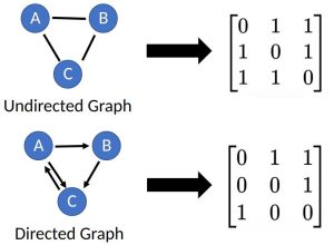
What is a Graph?

A graph, $G = (V,E)$ , is a data structure that consists of a set of nodes, $V$ , and a set of edges, $E$ . Graphs are used to represent connections (edges) between objects (nodes), where the edges can be directed or undirected depending on whether the relationships between the nodes have direction. An $n$ node graph can be represented by an $n \times n$ matrix, referred to as an adjacency matrix.

Idea of Distributed Vector Representations

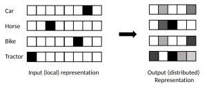
In machine learning architectures, the data input often needs to be converted to a tensor for the model, e.g. via 1-hot encoding. This provides an input (or local) representation of the data, which if we think about 1-hot encoding creates a large, sparse representation of 0s and 1s. The input representation is a discrete representation of objects, but lacks information on how things are correlated, how related they are, what they have in common. Often, machine learning models learn a distributed representation, where it learns how related objects are; nodes that are similar will have similar distributed representations. If each node is represented by an input vector, when the model learns a distributed vector, this is typically a much smaller vector. The diagram below gives a visual representation of how the model goes from a local to distributed representation [3]. As an example, the skip-gram model is a method which learns distributed vector representations to capture syntactic and semantic word relationships [4].

Brief Overview of what a Neural Network does

A neural network is a machine learning model comprised of interconnected nodes (called artificial neurons), which are organised into layers. These neurons process and transmit information through weighted connections, where the weights are tunable parameters. The layer-wise structure allows the mappings to create more and more abstract representations of the inputs. A classic example of a NN is for image classification. The NN is trained on a large dataset of images, where each image is labelled with a specific category, e.g. “dog” or “cat”. The NN learns the features and patterns in the images that help it to classify the image into a category. Then when presented with an unseen image, it will output probabilities of which category the image belongs to. They are trained in an iterative manner, and there are lots of adjustable choices for the model which can effect the prediction accuracy. By training NNs on large amounts of data to learn, they are useful to make predictions, classify data, and recognise patterns.

Graph Neural Networks (GNNs)

The inputs to a GNN are:

An $n \times d$ feature matrix of the nodes, $X$ ( $n$ nodes, $d$ input features). $X$ could for example be some 1-hot encoding matrix of features about the nodes.
An $n \times n$ adjacency matrix, $A$ .

You can think of a GNN as taking in an initial (input) representation of each node, $X$ , and a graph structure the nodes belong to, $A$ , and outputting some output representation of each node, $H$ . The initial representation has information about each node individually, and the output represents how each node belongs within the context of the graph given its features. The GNN exploits local interactions made by nodes to update the features of each node and maps to a latent feature space, $H$ . $H$ is an $n \times f$ matrix, where $f$ is the number of output features per node, which can be thought of as the distributed representation in the context of distributed vector representations. Usually $f << d$ .

$\underset{inputs}{(X, A)} \xrightarrow{\text{GNN}} \underset{outputs}{(H, A)}$

If you are familiar with embedding methods, you may think of $H$ as the embedding vectors of the graph after passing it through the GNN. Similar nodes will be closer to one another in the embedding space.

The data used for training the GNN is split like it would be for a NN, into a train-validation-test split. At each layer in the GNN, the values of $H$ are updated in a train-validation setup, and once all layers are passed through, the test data is used to evaluate the performance of the model. If there are $L$ layers of the GNN, then there are $L$ values of $H$ calculated, $H^{(0)}$ ,…, $H^{(L)}$ , where $H^{(0)} = X$ . But how is $H$ calculated?

Let’s start by considering the case where the graph $A$ is a binary undirected and unweighted graph – i.e. $A_{ij} = A_{ji} = \begin{cases} 0, & \text{if}\ i \leftrightarrow j \\ 1, & \text{otherwise} \end{cases}$ . Each neural network layer can be thought of as a non-linear function update of the previous layer:

$H^{(\ell +1)} = f(H^{(\ell)}, A)$

The particular GNN model choice is decided by the choice of $f(\cdot, \cdot)$ .

If we consider the simple update rule: $H^{(\ell+1)} = \sigma(A H^{(\ell)} W^{(\ell)})$ , where $W^{(\ell)}$ is a learnable node-wise shared linear transformation (the weight matrix for the $\ell^{th}$ layer) and $\sigma$ is a non-linear activation function (e.g. ReLU), this model encounters two limitations listed below. Most models which are used in practice make two adjustments to the input to circumvent possible problems/limitations:

If a node does not have a self loop in the graph ( $A_{ii} = 0$ ), when any matrix is multiplied with $A$ , for every node the feature vectors of all neighbouring nodes are summed up, but the node itself is not included. This means that the node is not considering the information it has about itself. To fix this, $A$ is updated to have every node connect to itself, by $\tilde{A} = A + I$ , where $I$ is the $n \times n$ identity matrix.
If $A$ or $\tilde{A}$ is multiplied by another matrix, it can change the scale of the output features. Therefore it is usual to normalise avoid this problem – e.g. multiplying $\tilde{A}$ by the degree matrix $\tilde{D}$ , where $\tilde{D}_{ii} = \sum\limits_j \tilde{A}_{ij}$ . This adjustment is sometimes referred as a mean pooling update rule.

A popular choice of GNN is the Graph Convolutional Network (GCN) [5]. We shall look at the update rules for this model in a bit more detail.

Graph Convolutional Network (GCN)

For this model, the input graph used is $\tilde{A}$ as described above, however the normalisation rule used is the symmetric normalisation: $\tilde{D}^{-\frac{1}{2}} \tilde{A} \tilde{D}^{-\frac{1}{2}}$ . The update rule for a GCN thus looks like:

$H^{(\ell+1)} = \sigma ( \tilde{D}^{-\frac{1}{2}} \tilde{A} \tilde{D}^{-\frac{1}{2}} H^{(\ell)} W^{(\ell)})$

where for each node this looks like:

$\textbf{h}_i^{(\ell+1)} = \sigma \left( \sum\limits_{j \in N_i} \frac{1}{\sqrt{|N_i||N_j|}} W^{(\ell)} \textbf{h}_j^{(\ell)} \right)$

$N_i$ denotes the set of neighbours of node $i$ . At each layer, node $i$ is being updated by a non-linear transformation ( $\sigma$ ) of the average of all its neighbours features in that layer. At the beginning each node knows about itself. In the first layer, it can learn about its distance 1 neighbours, in the second layer it begins to learn something about its distance 2 neighbours . At each layer the nodes learn more about how they belong in the graph, there is an increasing perceptive field of what you know about each node.

More generally, a GCN can be expressed as an explicit version of the below:

$\textbf{h}_i^{(\ell+1)} = \sigma \left( \sum\limits_{j \in N_i} \alpha_{ij} W^{(\ell)} \textbf{h}_j^{(\ell)} \right)$

where $\alpha_{ij}$ is explicitly defined as $\frac{1}{\sqrt{|N_i||N_j|}}$ in a GCN. $\alpha_{ij}$ says something about the importance of node $j$ ‘s features for node $i$ .

A popular benchmark/example of implementing GNNs is on the Cora dataset [6]. [6] describes the dataset as: “The Cora dataset consists of 2708 scientific publications classified into one of seven classes. The citation network consists of 5429 links. Each publication in the dataset is described by a 0/1-valued word vector indicating the absence/presence of the corresponding word from the dictionary. The dictionary consists of 1433 unique words.” There is a graph structure in the citation network and feature vectors for each node (of words in the dictionary) which can both be used in a GNN model. One example of use is to train the model to be able to classify papers that were not used to train the model into one of the seven classes based on the words present in their feature vector (words in the dictionary). [6] provides more examples of uses and comparisons of different GNN models based on their accuracy.

References

[1] Stokes, Jonathan M., et al. “A deep learning approach to antibiotic discovery.” Cell 180.4 (2020): 688-702.

[2] Fan, Wenqi, et al. “Graph neural networks for social recommendation.” The world wide web conference. 2019.

[3] MSR Cambridge, AI Residency Advanced Lecture Series. An Introduction to Graph Neural Networks: Models and Applications, 2020.

[4] Mikolov, Tomas, et al. “Distributed representations of words and phrases and their compositionality.” Advances in neural information processing systems 26 (2013).

[5] Kipf, Thomas N., and Max Welling. “Semi-supervised classification with graph convolutional networks.” arXiv preprint arXiv:1609.02907 (2016).

[6] https://paperswithcode.com/dataset/cora