
A post by Ed Davis, PhD student on the Compass programme.
Introduction
Today is a great day to be a data scientist. More than ever, our ability to both collect and analyse data allow us to solve larger, more interesting, and more diverse problems. My research focuses on analysing networks, which cover a mind-boggling range of applications from modelling vast computer networks [1], to detecting schizophrenia in brain networks [2]. In this blog, I want to share some of the cool research I have been a part of since joining the COMPASS CDT, which has to do with the analysis of dynamic networks.
Network Basics
A network can be defined as an ordered pair, ")


 \in E \\ 0, & (i,j) \not\in E \end{array}")
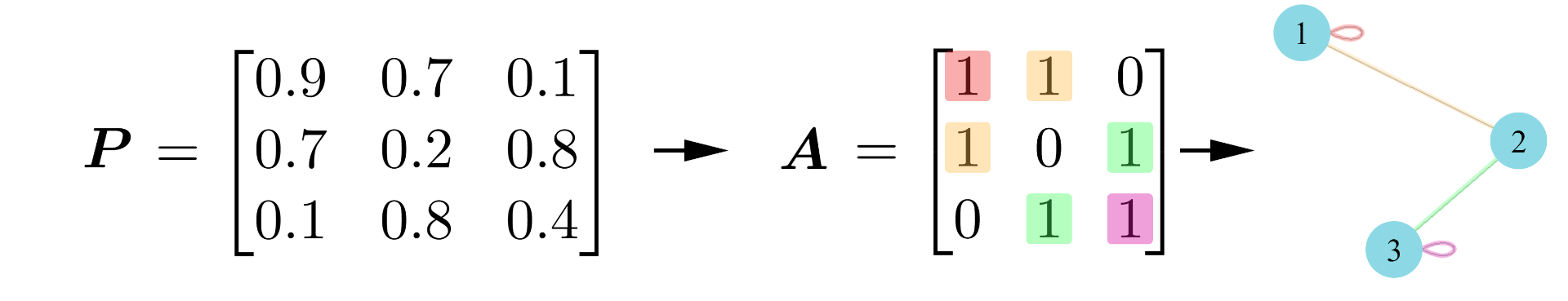
When we model networks, we can assume that there are some unobservable weightings which mean that certain nodes have a higher connection probability than others. We then observe these in the adjacency matrix with some added noise (like an image that has been blurred). Under this assumption, there must exist some unobservable noise-free version of the adjacency matrix (i.e. the image) that we call the probability matrix, 
")
where we have chosen a Bernoulli distribution as it will return either a 1 or a 0. As the connection probabilities are not uniform across the network (inhomogeneous) and the adjacency is sampled from some probability matrix (random), we say that 
Going a step further, we can model each node as having a latent position, which can be used to generate its connection probabilities and, hence define its behaviour. Using this, we can define node communities; a group of nodes that have the same underlying connection probabilities, meaning they have the same latent positions. We call this kind of model a latent position model. For example, in a network of social interactions at a school, we expect that pupils are more likely to interact with other pupils in their class. In this case, pupils in the same class are said to have similar latent positions and are part of a node community. Mathematically, we say there is a latent position 
![f: \mathbb{R}^k \times \mathbb{R}^k \rightarrow [0,1]](https://s0.wp.com/latex.php?latex=f%3A+%5Cmathbb%7BR%7D%5Ek+%5Ctimes+%5Cmathbb%7BR%7D%5Ek+%5Crightarrow+%5B0%2C1%5D&bg=ffffff&fg=000000&s=0 "f: \mathbb{R}^k \times \mathbb{R}^k \rightarrow [0,1]")
")
Under this model, our goal is then to estimate the latent positions by analysing
Network Embedding
Network embedding is a way of representing an 

- It allows us to only have to worry about a few feature vectors, as opposed to potentially thousands.
- By having a vector space representation, we open the flood gates for machine learning methods!
One simple, but very popular method of embedding is called spectral embedding. We start by taking the spectral decomposition (or eigendecomposition) of an adjacency matrix,

where 


Simple, right?
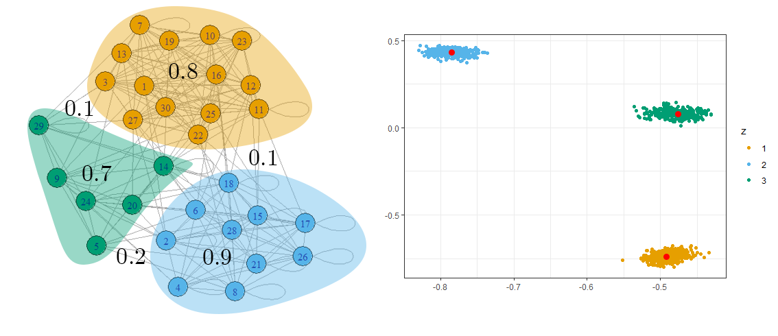
To demonstrate how effective this embedding is, Figure 2 shows an example network that features three communities of nodes (i.e. there are three distinct latent positions). By taking the spectral embedding of such a network, we can estimate the latent positions as the nodes will form Gaussian clusters around them.
Dynamic Network Embedding and Stability
We can capture a dynamic network through a series of adjacency matrices, }, \dots, \mathbf{A}^{(T)}\}")

- Longitudinal stability: if a node does not change its behaviour over time, it does not move in the embedding space,
.
- Cross-sectional stability: if node
behaves identically to another node
at some time
, then they are given the same position in the embedding space,
.
These conditions are natural because without longitudinal stability you cannot tell if a node is moving or stationary, and without cross-sectional stability, you cannot tell if any two nodes are behaving in the same way.
Recently, the research group that I am part of has developed a longitudinally and cross-sectionally stable dynamic embedding method known as the unfolded adjacency spectral embedding (or UASE) [3]. First, we construct a concatenation of all the adjacency snapshots, called the unfolded adjacency,
![\mathbf{A} = \left[\mathbf{A}^{(1)} | \dots | \mathbf{A}^{(T)} \right] \in \mathbb{R}^{n \times nT}](https://s0.wp.com/latex.php?latex=%5Cmathbf%7BA%7D+%3D+%5Cleft%5B%5Cmathbf%7BA%7D%5E%7B%281%29%7D+%7C+%5Cdots+%7C+%5Cmathbf%7BA%7D%5E%7B%28T%29%7D+%5Cright%5D+%5Cin+%5Cmathbb%7BR%7D%5E%7Bn+%5Ctimes+nT%7D&bg=ffffff&fg=000000&s=0 "\mathbf{A} = \left[\mathbf{A}^{(1)} | \dots | \mathbf{A}^{(T)} \right] \in \mathbb{R}^{n \times nT}")
Then we compute the spectral embedding of this unfolded adjacency matrix. As this matrix is rectangular, we cannot use spectral decomposition so instead we use the singular value decomposition and retain the top

where 


Real Data
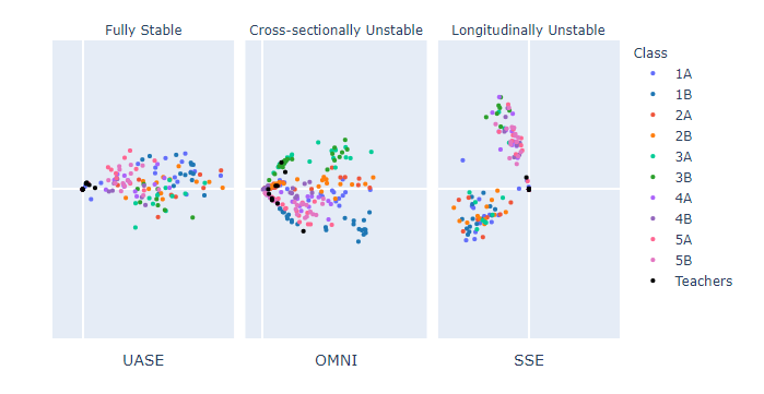
Now I’m going to demonstrate the importance of stability on some real data. The data set I have selected is a social interaction network of pupils and teachers at a French primary school as it exhibits significant periodic changes in structure as the day moves from class time to playtime [4]. We expect children and their teachers to only interact with others in their class during class time but may interact with anyone at break time.
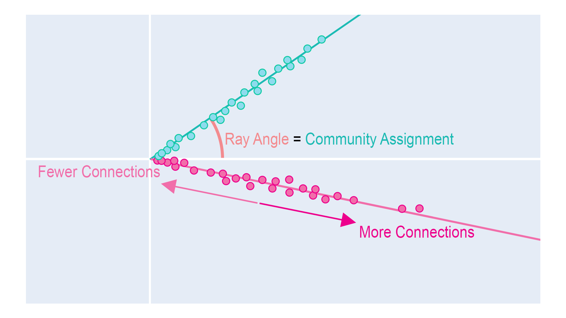
As with most real data, this data set is degree-heterogeneous; a way of saying that some nodes of the same community will have more interactions than others (these nodes are said to have a higher degree). So a very social pupil from class 1 will be further from the origin in the embedding space than a less social pupil in the same class. We, therefore, observe that nodes within the same community lie on a 1D subspace (which looks like a “ray”), with nodes with a higher activity further away from zero. During the class times, we expect our embeddings to have this ray structure.
Below is a figure with three different dynamic embedding methods. The separate spectral embedding (SSE) method computes a separate spectral embedding for each adjacency snapshot. The problem with doing this is that each time a new spectral embedding is calculated, the nodes are placed in a different space. This means that rays can appear to rotate significantly, even if they do not change their behaviour over time. This makes SSE a longitudinally unstable method. We can observe this problem below as colours representing the classes move wildly between time points (even during class times!), whereas the other two methods can display that node behaviour does not change significantly over class time (e.g. at 8 am and 9 am).
The omnibus embedding (or OMNI) computes a spectral embedding on a single matrix containing averages of all adjacency snapshots [2]. This allows it to be longitudinally stable as nodes remain in the same space over time. However, due to the averaging components of the matrix, it is not cross-sectionally stable. This problem is most apparent as we transition from class time (8 am and 9 am) to lunchtime (12 pm and 1 pm) as the class-like ray structure remains present, as opposed to UASE, despite people being able to freely interact with anyone. Only cross-sectionally stable methods can show such a significant change in network behaviour.
Conclusion
In conclusion, it is essential to use a fully stable dynamic embedding method to fully understand how a dynamic network changes over time. Now that we have a fully stable method in the form of the UASE, it’s exciting to see what we can discover in dynamic network datasets (of which there are many!) that previous unstable methods would not have been able to find.
References
[1] P. Rubin-Delanchy, “Manifold structure in graph embeddings,” https://arxiv.org/abs/2006.05168, 2021.
[2] K. Levin, A. Athreya, M. Tang, V. Lyzinski, and C. E. Priebe, “A central limit theorem for an omnibus embedding of random dot product graphs,” arXiv preprint arXiv:1705.09355, 2017.
[3] I. Gallagher, A. Jones, and P. Rubin-Delanchy, “Spectralembedding for dynamic networks with stability guarantees,”arXiv preprint arXiv:2106.01282, 2021.
[4] Ryan A. Rossi and Nesreen K. Ahmed, “The Network Data Repository with Interactive Graph Analytics and Visualization”, https://networkrepository.com/ia-primary-school-proximity-attr.php, 2015.