stability – Compass Blog

A post by Ed Davis, PhD student on the Compass programme.

Introduction

Today is a great day to be a data scientist. More than ever, our ability to both collect and analyse data allow us to solve larger, more interesting, and more diverse problems. My research focuses on analysing networks, which cover a mind-boggling range of applications from modelling vast computer networks [1], to detecting schizophrenia in brain networks [2]. In this blog, I want to share some of the cool research I have been a part of since joining the COMPASS CDT, which has to do with the analysis of dynamic networks.

Network Basics

A network can be defined as an ordered pair, $(V, E)$ , where $V$ is a node (or vertex) set and $E$ is an edge set. From this definition, we can represent any $n$ node network in terms of an adjacency matrix, $A \in \mathbb{R}^{n \times n}$ , where for nodes $i, j \in V$ ,

$A_{ij} = \Bigg\{ \begin{array}{ll} 1 & (i,j) \in E \\ 0, & (i,j) \not\in E \end{array}$ .

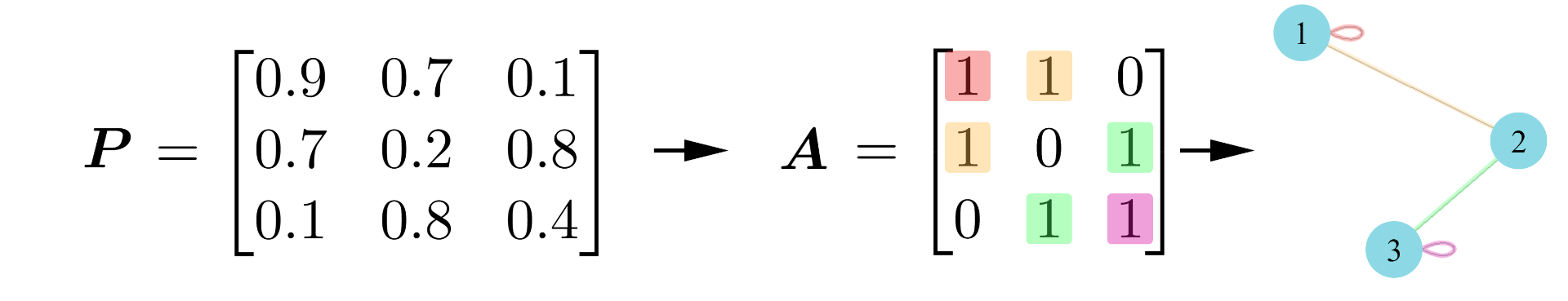
When we model networks, we can assume that there are some unobservable weightings which mean that certain nodes have a higher connection probability than others. We then observe these in the adjacency matrix with some added noise (like an image that has been blurred). Under this assumption, there must exist some unobservable noise-free version of the adjacency matrix (i.e. the image) that we call the probability matrix, $\mathbf{P} \in \mathbb{R}^{n \times n}$ . Mathematically, we represent this by saying

$A_{ij} \overset{\text{ind}}{\sim} \text{Bernoulli} \left(P_{ij} \right)$ ,

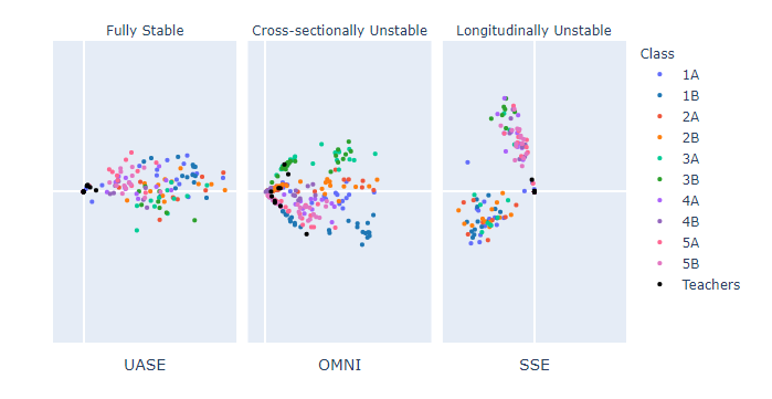
where we have chosen a Bernoulli distribution as it will return either a 1 or a 0. As the connection probabilities are not uniform across the network (inhomogeneous) and the adjacency is sampled from some probability matrix (random), we say that $\mathbf{A}$ is an inhomogeneous random graph.

*Figure 1: An inhomogeneous random graph. From some probability matrix, we draw an adjacency matrix that represents a network.*

Going a step further, we can model each node as having a latent position, which can be used to generate its connection probabilities and, hence define its behaviour. Using this, we can define node communities; a group of nodes that have the same underlying connection probabilities, meaning they have the same latent positions. We call this kind of model a latent position model. For example, in a network of social interactions at a school, we expect that pupils are more likely to interact with other pupils in their class. In this case, pupils in the same class are said to have similar latent positions and are part of a node community. Mathematically, we say there is a latent position $\mathbf{Z}_i \in \mathbb{R}^{k}$ assigned to each node, and then our probability matrix will be the gram matrix of some kernel, $f: \mathbb{R}^k \times \mathbb{R}^k \rightarrow [0,1]$ . From this, we generate our adjacency matrix as

$A_{ij} \overset{\text{ind}}{\sim} \text{Bernoulli}\left( f \left\{ \mathbf{Z}_i, \mathbf{Z}_j \right\} \right)$ .

Under this model, our goal is then to estimate the latent positions by analysing $\mathbf{A}$ .

Network Embedding

(more…)

Tag: stability

Student Perspectives: The Importance of Stability in Dynamic Network Analysis

Introduction

Network Basics

Network Embedding