A post by Daniel Williams, Compass PhD student.

Imagine that you are employed by Chicago’s city council, and are tasked with estimating where the mean locations of reported crimes are in the city. The data that you are given only goes up to the city’s borders, even though crime does not suddenly stop beyond this artificial boundary. As a data scientist, how would you estimate these centres within the city? Your measurements are obscured past a very complex border, so regular methods such as maximum likelihood would not be appropriate.

Chicago Homicides — **Figure 1:** Homicides in the city of Chicago in 2008. Left: locations of each homicide. Right: a density estimate of the same crimes, highlighting where the ‘hotspots’ are.

This is an example of a more general problem in statistics named truncated probability density estimation. How do we estimate the parameters of a statistical model when data are not fully observed, and are cut off by some artificial boundary?

The Problem

Incorporation of this boundary constraint into estimation is not straightforward. There are many factors which must be considered which make regular methods infeasible, we require:

knowledge of the normalising constant in a statistical model, which is unknown in a truncated setting;
incorporation of weighting points that are more ‘affected’ by the truncation.

A statistical model (a probability density function involving some parameters $\theta$ ) is defined as:

$p(x; \theta) = \frac{1}{Z(\theta)} \bar{p}(x;\theta).$

This is made up of two components: $\bar{p}(x; \theta)$ , the unnormalised part of the model, which is known analytically; and $Z(\theta)$ , the normalising constant, which is oftentimes unknown or undefinable. The goal of estimation is to find a vector of parameters $\theta$ which characterises our model, and makes the model resemble the data as closely as possible. Usually, we can estimate $\theta$ by trying to minimise the difference between the model, $p(x;\theta)$ , and the theoretical data density, $q(x)$ .

A Recipe for a Solution

Ingredient #1: Score Matching

A novel estimation method called score matching enables estimation even when the normalising constant, $Z(\theta)$ , is unknown. Score matching begins by taking the derivative of the logarithm of the probability density function, i.e.,

$\nabla_x \log p(x; \theta) = \nabla_x \log \bar{p}(x;\theta),$

which has become known as the score function. When taking the derivative, the dependence on $Z(\theta)$ is removed. To estimate the parameter vector $\theta$ , we can minimise the difference between $q(x)$ and $p(x;\theta)$ by minimising the difference between the two score functions, $\nabla_x \log p(x; \theta)$ and $\nabla_x \log q(x)$ . One such distance measure is the expected squared distance, so that score matching aims to minimise

$\mathbb{E} [\| \nabla_x \log p(x; \theta) - \nabla_x \log q(x)\|_2^2].$

With this first ingredient, we have eliminated the requirement that we must know the normalising constant.

Ingredient #2: A Weighting Function

Heuristically, we can imagine our weighting function should vary with how close a point is to the boundary. To satisfy score matching assumptions, we require that this weighting function $g(x)$ must have the property that $g(x') = 0$ for any point $x'$ on the boundary. A natural candidate would be the Euclidean distance from a point $x$ to the boundary, i.e.,

$g(x) = \|x - \tilde{x}\|_2, \qquad \tilde{x} = \text{argmin}_{x'\text{ in boundary}} \|x - x'\|_2.$

This easily satisfies our criteria. The distance is going to be exactly zero on the boundary itself, and will approach zero the closer the points are to the edges.

Ingredient #3: Any Statistical Model

Since we do not require knowledge of the normalising constant through the use of score matching, we can choose any probability density function $p(x; \theta)$ that is appropriate for our data. For example, if we are modelling count data, we may choose a Poisson distribution. If we have some sort of centralised location data, such as in the Chicago crime example in the introduction, we may choose a multivariate Normal distribution.

Combine Ingredients and Mix

We aim to minimise the expected distance between the score functions, and we weight this by our function $g(x)$ , to give

$\min_{\theta} \mathbb{E} [g(x) \| \nabla_x \log p(x; \theta) - \nabla_x \log q(x)\|_2^2].$

The only unknown in this equation now is the data density $q(x)$ (if we knew the true data density, there would be no point in estimating it with $p(x;\theta)$ ). However, we can rewrite this equation using integration by parts as

$\min_{\theta} \mathbb{E} \big[ g(x) [\|\nabla_x \log p(x; \theta)\|_2^2 + 2\text{trace}(\nabla_x^2 \log p(x; \theta))] + 2 \nabla_x g(x)^\top \nabla_x \log p(x;\theta)\big].$

This can be numerically minimised, or if $p(x; \theta)$ is in the exponential family, analytically minimised to obtain estimates for $\theta$ .

Results

Artificial Data

As a sanity check for testing estimation methods, it is often reassuring to perform some experiments on simulated data before moving to real world applications. Since we know the true parameter values, it is possible to calculate how far our estimated values are from their true counterparts, thus giving a way to measure estimation accuracy.

Pictured below in Figure 2 are two experiments where data are simulated from a multivariate normal distribution with mean $\mu = [1, 1]$ and known variance $\sigma^2 = 1$ . Our aim is to estimate the parameter $\theta$ to be close to $[1,1]$ . The red crosses in the image are the true means at $[1,1]$ , and the red dots are the estimates given by truncated score matching.

**Figure 2 (a):** Points are only visible around a unit ball from [0,0].

**Figure 2 (b):** Points are only visible inside a box to the left of the mean.

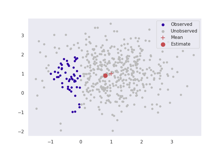
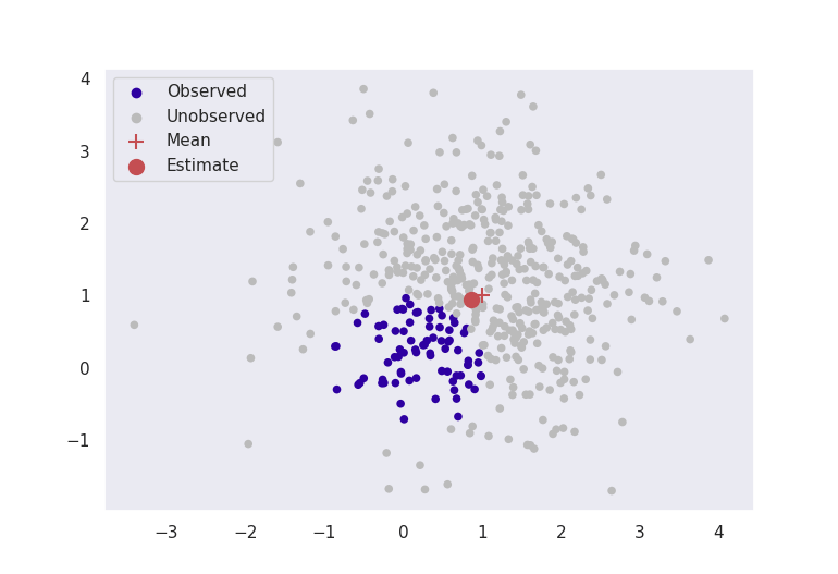
These figures clearly indicate that in this basic case, this method is giving sensible results. Even by ignoring most of our data, as long as we formulate our problem correctly, we can still get accurate results for estimation.

Chicago Crime

Now we come back to the motivating problem, and the task is to estimate the centres of police reported crime in the city of Chicago, given the longitudes and latitudes of homicides in 2008. Our specification changes somewhat:

from the original plots, it seems like there are two centres, so the statistical model we choose is a 2-dimensional mixed multivariate Normal distribution;
the variance is no longer known, but to keep estimation straightforward, the standard deviation $\sigma$ is fixed so that $2\sigma$ roughly covers the ‘width’ of the city.

Figure 3 below shows applying this method to this application.

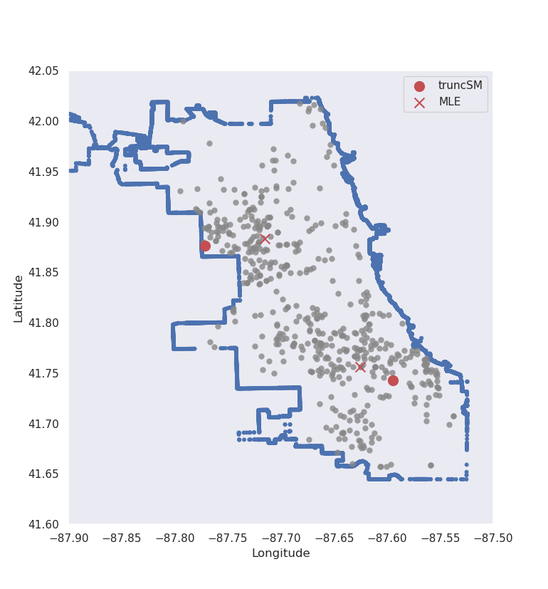
**Figure 3:** Estimates of two crime centres in Chicago for truncated score matching (truncSM) and maximum likelihood estimation (MLE).

Truncated score matching has placed its estimates for the means in similar, but slightly different places than standard MLE. Whereas the maximum likelihood estimates are more central to the truncated dataset, the truncated score matching estimates are placed closer to the outer edges of the city. For the upper-most crime centre, around the city border the data are more ‘tightly packed’ – which is a property we expect of multivariate normal data. This result does not reflect the true likelihood of crime in a certain neighbourhood, and has only been presented to provide a visual explanation of the method. The actual likelihood depends on various characteristics in the city that are not included in our analysis, see here for more details.

Final Thoughts

Score matching is a powerful tool, and by not requiring any form of normalising constant, enables the use of some more complicated models. Truncated probability density estimation is just one such example of an intricate problem which can be solved with this methodology, but it is one with far reaching and interesting applications. Whilst this blog post has focused on location-based data and estimation, truncated probability density estimation could have a range of applications. For example, consider disease/virus modelling such as the COVID-19 pandemic. The true number of cases is obscured by the number of tests that can be performed, so the density evolution of the pandemic through time could be fully modelled with incorporation of this constraint using this method. Other applications as well as extensions to this method will be fully investigated in my future PhD projects.

Some Notes

Alternative methods which do not require the normalising constant: We could choose a model which has truncation built into its specification, such as the truncated normal distribution. For complicated regions of truncation, such as the city of Chicago, it is highly unlikely that an appropriate model specification is available. We could also perform some rejection algorithm to approximate the normalising constant, such as MCMC or ABC, but these are often very slow, and do not provide an exact solution. Score matching can have an analytical estimate for exponential family models, and even when it does not, minimisation is usually straightforward and fast.

Choice of the weighting function: We did not need to specify $g(x)$ before formulating our score matching objective function in ingredient #3. In fact, under some assumptions (the function $g(x)$ is 1-Lipschitz continuous) it can be shown that the choice of $g(x)$ which gives the supremum of the score matching expectation is in fact the Euclidean distance which was specified earlier, so it was not just a heuristic!

Score matching derivation conditions: This post has hand-waved some conditions of the derivation of the score matching objective function. There are two conditions which must be satisfied in the weighting function $g(x)$ so that the integration by parts ‘trick’ can work correctly. Firstly, $g(x)$ must be positive for every $x$ . Secondly, for any $x'$ in the boundary, $g(x') = 0$ . For more information, see the further reading section below.

Student perspectives: How can we do data science without all of our data?