
Tag: University of Bristol
Advai: DataScience@work seminar
Student Perspectives: Avoiding our problems ~ Noise Contrastive Estimation
A post by Henry Bourne, PhD student on the Compass programme.
Currently I’ve been researching Noise Contrastive Estimation (NCE) techniques for representation learning aided by my supervisor Dr. Rihuan Ke. Representation learning concerns itself with learning low-dimensional representations of high-dimensional data that can then be used to quickly solve a general downstream task, eg. after learning general representations for images you could quickly and cheaply train a classification model on top of the representations.
NCE is a general estimator for parametrised probability models as I will explain in this blogpost. However, it can also be cleverly used to learn useful representations in an unsupervised (or equivalently self-supervised) manner, which I will also explain. I’ll start by explaining the problem that NCE was created to solve, then provide a quick comparison to other methods, explain how researchers have built on this method to carry out representation learning and finally discuss what I am currently working on.
NCE solves the problem of computing a normalising constant by avoiding the problem altogether and solving some other proxy problem. Methods that are able to model unnormalised probability models are known as Energy Based Models (EBM’s). We will begin by describing the problem with the normalising constant before getting on to how we will avoid it.
The problem … with the normalising constant
Let’s say we have some arbitrary probability distribution, $p_{d}(\cdot)$, and a parametrised probability model, $p_{m}(\cdot ; \alpha)$, which we would like to accurately model the underlying probability distribution. Let’s further assume that we’ve picked our model well such that $\exists \alpha^{*}$ such that $p_{d}(\cdot) = p_{m}(\cdot ; \alpha^{*})$.
Let’s just fit it to our data sampled from the underlying distribution using Maximum Likelihood Estimation! Sounds like a good idea, MLE has been extensively used, is reliable, is efficient and achieves the Cramer-Rao lower bound (the lowest possible bound an unbiased estimator can achieve for its variance/MSE), is asymptotically normal, is consistent, is unbiased and doesn’t assume normality. Moreover, there are a lot of tweaked MLE techniques out there that you can use if you would like an estimator with slightly different properties.
First let’s look under the hood of our probability model, we can write it as so:
$
\begin{array}{l|l}
p_{m}(\cdot;\alpha)=\frac{p_{m}^{0}(\cdot; \alpha)}{Z(\alpha)} & \text{where,} \: Z(\alpha) = \int p_{m}^{0}(u; \alpha) du
\end{array}
$
The likelihood is our probability model for some $\alpha$ evaluated over our dataset. Evaluating the likelihood becomes tricky when there isn’t an analytical solution for the normalisation term, $Z(\alpha)$, and the possible set of values $u$ can take becomes large. For example if we would like to learn a probability distribution over images then this normalisation term becomes intractable.
By working with the log we get better numerical stability, it makes things easier to read and it makes calculations and taking derivatives easier. So, let’s take the log of the above:
| $ \begin{aligned} &{} p_{m}(\cdot;\alpha) = \frac{p_{m}^{0}(\cdot; \alpha)}{Z(\alpha)} \\ & \Rightarrow \log p_{m}(\cdot; \theta) = \log p_{m}^{0} (\cdot ; \alpha) +c \end{aligned} $ |
$\text{Where, } \\ \theta = \{\alpha, c \}, \\ \text{c an estimate of} -\log Z(\alpha)$ |
Where, we write $p_{m}^{0}(\cdot;\alpha)$ to represent our unnormalized probability model. After taking the $\log$ we can write our normalising constant as $c$ and then include it as a parameter of our model. So, our new model now parameterised by $\theta$, $p_{m}(\cdot;\theta)$, is self-normalising, ie. it estimates it’s normalising constant. Another approach to make the model self-normalising would be to simply set $c=0$, implicitly making the model self-normalising. This is what is normally done in practice, but it assumes that your model is complex enough to be able to indirectly model $c$.
Couldn’t we just use MLE to estimate $\log p_{m}(\cdot ; \theta)$? No we can’t! This is because the likelihood can be made arbitrarily large by making $c$ large.
This is where Noise Contrastive Estimation (NCE) comes in. NCE has been shown theoretically and empirically to be a good estimator when taking this self-normalizing assumption. We’ll assess it versus competing methods at the end of the blogpost. But before we do that let’s first describe the original NCE method named binary-NCE [1] later we will mention some of the more complex versions of this estimator.
Binary-NCE
The idea with binary-NCE [1] is that by avoiding our problems we fix our problems! ie. We would like to create and solve an ‘easier’ proxy problem which in the process solves our original problem.
Let’s say we have some noise-distribution, $p_{n}(\cdot)$, which is easy to sample from, allows for an analytical expression of $\log p_{n} (\cdot)$ and is in some way similar to our $p_{d}(\cdot)$ (our underlying probability distribution which we are trying to estimate). We would also like $p_{n}(\cdot)$ to be non-zero wherever $p_{d}(\cdot)$ is non-zero. Don’t worry too much about these assumptions as they are normally quite easy to satisfy, apart from an analytical expression being available. They just are necessary for our theoretical properties to hold and for binary-NCE to work in practice.
We would like to create and solve a proxy problem where given a sample we would like to classify whether it was drawn from our probability model or from our noise distribution. Consider the following density ratio.
$
\begin{aligned}
\frac{p_{m}(u;\alpha)}{p_{n}(u)}
\end{aligned}
$
\begin{aligned}
\frac{p_{m}(u;\alpha)}{p_{n}(u)}
\end{aligned}
$
If this density ratio is bigger than one then it means that $u$ is more likely to have come from our probability model, $p_{m}(\cdot;\alpha)$. If it is smaller than one then $u$ is more likely to have come from our noise distribution, $p_{n}(\cdot)$. Therefore, if we can model this density ratio then we will have a model for how likely a sample is to have come from our probability model as opposed to have being sampled from our noise distribution.
Notice that we are modelling our normalised probability model above, we can rewrite it in terms of our unnormalised probability model as follows.
$
\begin{aligned}
& \log \left(\frac{p_{m}(u;\alpha)}{p_{n}(u)} \right) \\
& = \log \left(\frac{p_{m}^{0}(u;\alpha)}{Z(\alpha)} \cdot \frac{1}{p_{n}(u)} \right) \\
& = \log \left(\frac{p_{m}^{0}(u;\alpha)}{p_{n}(u)} \right) +c \\
& = \log p_{m}^{0}(u;\alpha) + c – \log p_{n}(u) \\
& = \log p_{m}(u;\theta) – \log p_{n}(u)
\end{aligned}
$
Let’s now define a score function $s$ that we will use to model our rewrite of the density ratio just above:
$
\begin{aligned}
s(u;\theta) = \log p_{m}(u;\theta) – log p_{n}(u)
\end{aligned}
$
One further step before introducing our objective function. We would like to model our score function somewhat as a probability, we would also like our model to not just increase the score indefinitely. So we will put our modelled density ratio through the sigmoid/ logistic function.
$
\begin{aligned}
\sigma(s(u;\theta)) = \frac{1}{1+ \exp(-s(u;\theta))}
\end{aligned}
$
We would like to classify according to our model of the density ratio whether the sample is ‘real’ / ‘positive or just ‘noise’/ ‘fake’/ ‘negative’. So a natural choice for the objective function is the cross-entropy loss.
$
\begin{aligned}
J(\theta) = \frac{1}{2N} \sum_{n} \log [ \sigma(s(x_{n};\theta))] + \log [1- \sigma(s(x_{n}’;\theta))]
\end{aligned}
$
Where $x_{i} \sim p_{d}$, $x_{i}’ \sim p_{n}$ for $i \in \{1,…,N\}$. Here we simply assume one noise sample per observation, but we can trivially extend it to any integer $K>0$ and in fact asymptotically the estimator gets better performance as we increase K.
Once we’ve estimated our density ratio we can easily recover our normalised probability model of the underlying distribution by adding the log probability density of the noise function and taking the exponential.
This estimator is consistent, efficient and asymptotically normal. In [1] they also showed it working empirically in a range of different settings.
How does it compare to other estimators of unnormalised parameterised probability density models?
NCE is not the only method we can use to solve the problem of estimating an unnormalised parameterised probability model. As we mentioned NCE belongs to a family of methods named Energy Based Models (EBM’s) which all aim to solve this very problem of estimating an unnormalised probability model. Let’s very briefly mention some of the alternatives from this family of methods, please do check out the references in this sub-section if you would like to learn more. We will talk about the methods as they appeared in their seminal form.
One alternative is called contrastive divergence which estimates an unnormalised parametrised probability model by using a combination of MCMC and the KL divergence. Contrastive Divergence was originally introduced with Boltzmann machines in mind [9], MCMC is used to generate samples of the activations of the Boltzmann machine and then the KL divergence measures the difference between the distribution of the activations given by the real data and the simulated activations. We then aim to minimise the KL divergence.
Score matching [11] models a parameterised probability model without the computation of the normalising term by estimating the gradient of the log density which it calls the score function. It does this by minimising the expected square distance between the score function and the score function of the observed data. However, obtaining the score function of the observed data requires estimating a non-parametric model from the data. They magically avoid doing this by deriving an alternative form of the objective function, through partial integration, leaving only the computation of the score function and it’s derivative.
Importance sampling [10], which has been around for quite a while uses a weighted version of MCMC to focus on parts of the distribution that are ‘more important’ and in the process self-normalises. Which makes it better than regular MCMC because you can use it on unnormalised probability models and it should be more efficient and have lower variance.
[1] contains a simple comparison between NCE, contrastive divergence, importance sampling and score matching. In their experimental setting they found contrastive divergence got the best performance, closely followed by NCE. They also measured computation time and found NCE to be the best in terms of error versus computation time. This by no means crowns NCE as the best estimator but is a good suggestion as to it’s utility, so is the countless ways it’s been used with high efficacy on a multitude of real-world problems.
Building on Binary-NCE (Ranking-NCE and Info-NCE)
Taking inspiration from Binary-NCE a number of other estimators have been devised. One such estimator is Ranking-NCE [2]. This estimator has two important elements.
The first is that the estimator assumes that we are trying to model a conditional distribution, for example $p(y|x)$. By making this assumption our normalising constant is different for each value of the random variable we are conditioning on, ie. Our normalising term is now some $Z(x;\theta)$ and we have one for each possible value of x. This loosens the constraints on our estimator as we don’t require our optimal parameters, $\theta^{*}$, to satisfy $\log Z(x;\theta^{*}) = c$ for some $c$ for all possible values of $x$. This means we can apply our model to problems where the number of possible values of $x$ is much larger than the number of parameters in our model. For further details on this please refer to [2], section 2.
The second is that it has an objective that given an observed sample $x$, and an integer $K>1$ samples from the noise distirbution, the objective ranks the samples in order of how likely they were to have come from the model versus the noise distribution. Again for further details please refer to [2].
Importantly this version of the estimator can be applied to more complex problems and empirically has been shown to achieve better performance.
Now what we’ve been waiting for … how can we use NCE for representation learning? This is where Info(rmation) NCE comes in. It essentially is Ranking-NCE but we chose our conditional distribution and noise distribution in a specific way.
We consider a conditional probability of the form p(y|x) where $y \in \mathbb{R}^{d_{y}}$, $x \in \mathbb{R}^{d_{x}}$, $d_{y} < d_{x}$. Where $x$ is some data and $y$ is the low-dimensional representation we would like to learn for $x$. We then choose our noise distribution, $p_{n}$, to be the marginal distribution of our representation $y$, $p_{y}$. So our density ratio becomes.
$
\begin{aligned}
\frac{p_{m}(y|x; \theta)}{p_{y}(y)}
\end{aligned}
$
This is now a measure of how likely a given $y$ is to have come from the conditional distribution we are trying to model, ie. how likely is this representation to have been obtained from $x$, versus being some randomly sampled representation.
A key thing to notice is that we are unlikely to have an analytical form of the $log$ of the marginal distribution of $y$. In fact, this doesn’t matter as we aren’t actually interested in modelling the conditional distribution in this case. What we are interested in is the fact that by employing a Ranking-NCE style estimator and modelling the above density ratio we maximise a lower bound on the mutual information between $Y$ and $X$, $I(Y;X)$. A proof for this along with the actual objective function can be found in [3].
This is quite an amazing result! We solve a proxy problem of a proxy problem and we get an estimator with great theoretical guarantees that is computationally efficient that maximises a mutual information which allows us to, in an unsupervised manner, learn general representations for data. So we avoid our problems twice! I appreciate that above were two big jumps with not much detail but I hope it gives a sense as to the link between NCE in it’s basic form and representation learning. More specifically, NCE is known as a self-supervised learning method which simply means an unsupervised method which uses supervised methods but generates its own teaching signal. Even more specifically, NCE is a contrastive method which gets its name from the fact that it contrasts samples against each other in order to learn. The other popular category of self-supervised learning methods are called generative models, you may have heard of these!
My Research
Now we know a little bit about NCE and how we can use it to do representation learning, what am I researching?
Info-NCE has been applied with great success in many self-supervised representation learning techniques, a good one to check out is [4]. Contrastive self-supervised learning techniques have been shown to outperform supervised learning in many areas. They also solve some of the key challenges that face generative representation learning techniques in more challenging domains than language such as images and video. This review [5] is a good starting point for learning more about what contrastive learning and generative learning are and some of their differences.
However, there are still lots of problem areas where applying NCE, without very fancy neural network architectures and techniques, doesn’t do so well or outright fails. Moreover, many of these techniques introduce extra requirements on memory, compute or both. Additionally, they can often be highly complex and their ablation studies are poor.
Currently, I’m looking at applying new kinds of density ratio estimation methods to representation learning, in a similar way to info-NCE. These new density ratio estimation techniques when applied in the correct way will hopefully lead to representation learning techniques that are more capable in problem areas such as multi-modal learning [6], multi-task learning [7] and continual learning [8].
Currently, of most interest to me is multi-modal learning. This is concerned with learning a joint representation over data comprised of more than one modality, eg. text and images. By being able to learn representations on data consisting of multiple modalities it’s possible to learn higher quality representations (more information) and makes us capable of solving more complex tasks that require working over multiple modalities, eg. most robotics tasks. However, multi-modal learning has a unique set of difficult challenges that make naively using representation learning techniques on it challenging. One of the key challenges is balancing a trade-off between learning to construct representations that exploit the synergies between the modalities and not allowing the quality of the representations to be degraded by the varying quality and bias of each of the modalities. We hope to solve this problem in an elegant and simple manner using density ratio estimation techniques to create a novel info-NCE style estimator.
Hope you enjoyed! If you would like to reach me or read some of my other blogposts (I have some more in-depth ones about NCE coming out soon) then checkout my website at /phd.h-0-0.com.
References
[1] :
Gutmann, M. and Hyvärinen, A., 2010, March. Noise-contrastive estimation: A new estimation principle for unnormalized statistical models. In Proceedings of the thirteenth international conference on artificial intelligence and statistics (pp. 297-304). JMLR Workshop and Conference Proceedings.
[2] :
Ma, Z. and Collins, M., 2018. Noise contrastive estimation and negative sampling for conditional models: Consistency and statistical efficiency. arXiv preprint arXiv:1809.01812.
[3] :
Oord, A.V.D., Li, Y. and Vinyals, O., 2018. Representation learning with contrastive predictive coding. arXiv preprint arXiv:1807.03748.
[4] :
Chen, T., Kornblith, S., Norouzi, M. and Hinton, G., 2020, November. A simple framework for contrastive learning of visual representations. In International conference on machine learning (pp. 1597-1607). PMLR.
[5] :
Liu, X., Zhang, F., Hou, Z., Mian, L., Wang, Z., Zhang, J. and Tang, J., 2021. Self-supervised learning: Generative or contrastive. IEEE transactions on knowledge and data engineering, 35(1), pp.857-876.
[6] :
Baltrušaitis, T., Ahuja, C. and Morency, L.P., 2018. Multimodal machine learning: A survey and taxonomy. IEEE transactions on pattern analysis and machine intelligence, 41(2), pp.423-443.
[7] :
Zhang, Y. and Yang, Q., 2021. A survey on multi-task learning. IEEE Transactions on Knowledge and Data Engineering, 34(12), pp.5586-5609.
[8] :
Wang, L., Zhang, X., Su, H. and Zhu, J., 2024. A comprehensive survey of continual learning: Theory, method and application. IEEE Transactions on Pattern Analysis and Machine Intelligence.
[9] :
Carreira-Perpinan, M.A. and Hinton, G., 2005, January. On contrastive divergence learning. In International workshop on artificial intelligence and statistics (pp. 33-40). PMLR.
[10] :
Kloek, T. and Van Dijk, H.K., 1978. Bayesian estimates of equation system parameters: an application of integration by Monte Carlo. Econometrica: Journal of the Econometric Society, pp.1-19.
[11] :
Hyvärinen, A. and Dayan, P., 2005. Estimation of non-normalized statistical models by score matching. Journal of Machine Learning Research, 6(4).
Student Perspectives: What is Confounding?
A post by Emma Tarmey, PhD student on the Compass programme.
This blog post serves as an introduction to the problem of confounder handling within the broader topic of covariate selection and model selection for causal inference purposes. In this post, we begin with a motivating example, describe the problem of confounding, describe current solutions to the problem and how statistical solution methods compare to knowledge-based solution methods. It is intended that readers come away from this article understanding which use cases each of the solution methods are intended for, as well as what advantages and disadvantages each method provides.
Introduction
There exists a common saying, “correlation does not imply causation”. This phrase is often used when discussing statistical analyses to describe the idea that just because two phenomena or patterns often appear together, does not automatically mean that one necessarily causes the other. There are a number of reasons why two events, A and B, may occur together, with “A causes B” being only one of several explanations for the observed correlation. In epidemiology, substantiating a causal claim, “causal inference”, can be highly valuable towards determining medical best practice and testing the effectiveness of medical treatments and interventions. A correlation between two events, A and B, may be distorted or even fabricated whole-cloth by the influence of an outside event C, which mutually causes both. As such, particularly in the context of clinical trials for medical treatments, verifying that no such outside influences are distorting our results is essential for producing valid causal inferences.
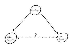
Yellow Fingers and Lung Cancer
To motivate the idea of a distorted correlation from the introduction, we look to a famous example: the association between the yellowing at the tip’s of ones fingers and incidence of lung cancer.[1][2] We observe from the literature that, when attempting to predict incidence of lung cancer, the yellowing of ones finger tips makes an excellent predictor variable.[1] However, there is no causal link between these two events, instead, both the yellowing and lung cancer are mutually caused by smoking.[2] This, in turn, creates an unhelpful statistical association between the two variables, one which is then correctly estimated in modelling but no longer corresponds just to our causal pathway. As such, when attempting to understand causal factors to lung cancer, it becomes important not to declare yellowing as a cause despite the fact that yellowing may “look like a cause” based on the data itself.
One can imagine, in an isolated example like this, it can be straight-forward to detect this from first principles using the existing causal knowledge we have. But, if for example a given study has not recorded smoking as a variable, we become unable to identify the phenomenon and thus unable to correctly attribute the source of our statistical associations. The phenomenon within causal structures of a common cause is referred to as “confounding”, thus giving us the sub-problem of “confounder handling” when attempting to use our statistical models for causal inference. Notably, causal pathways can be more complex than the above example. If we have a longer pathway by which we add to the statistical association between X and Y, any such covariate on that pathway is a potential confounder, whose adjustment will solve our problem. We define our problem formally as follows:
Problem: Confounder Handling
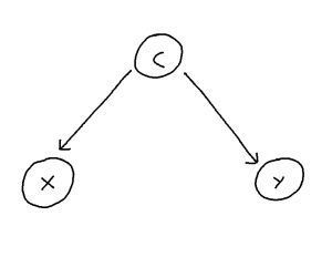
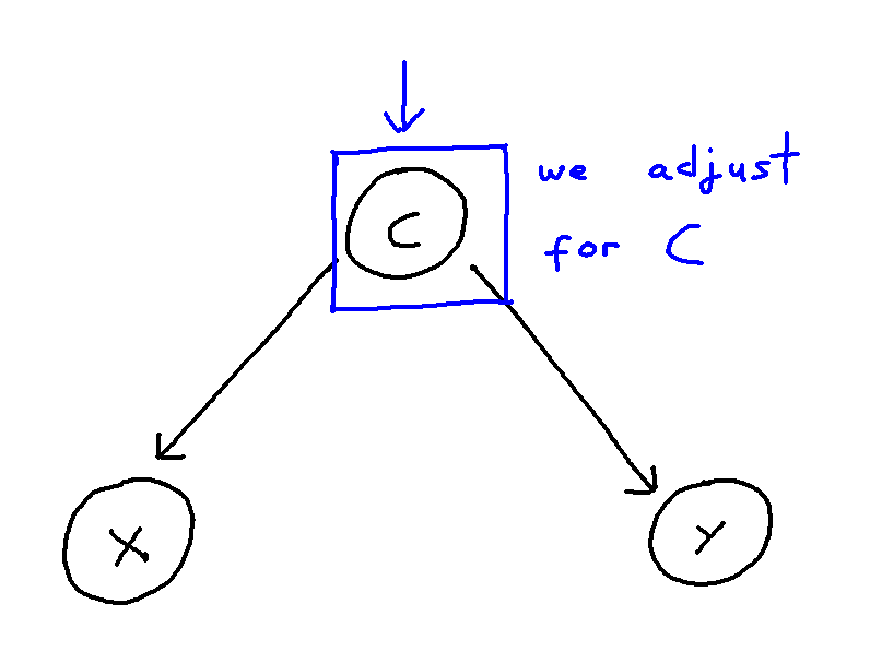
Confounding is defined as the phenomenon within any causal structure wherein both an exposure (input variable) and outcome (output variable) are mutually caused by a third outside variable (the confounder). This in turn creates a statistical association between the two covariates which is not attributable to a causal pathway from X to Y. This phenomenon takes the following general shape:
It can be helpful to think of confounder-handling as containing two sub-problems which we solve together:
- Confounder Identification: Identifying the set of all covariates which act as confounders within a given causal structure
- Control-Set Selection: Selecting an optimal (by some criterion) subset of these identified confounders to include in the model to best control for confounding
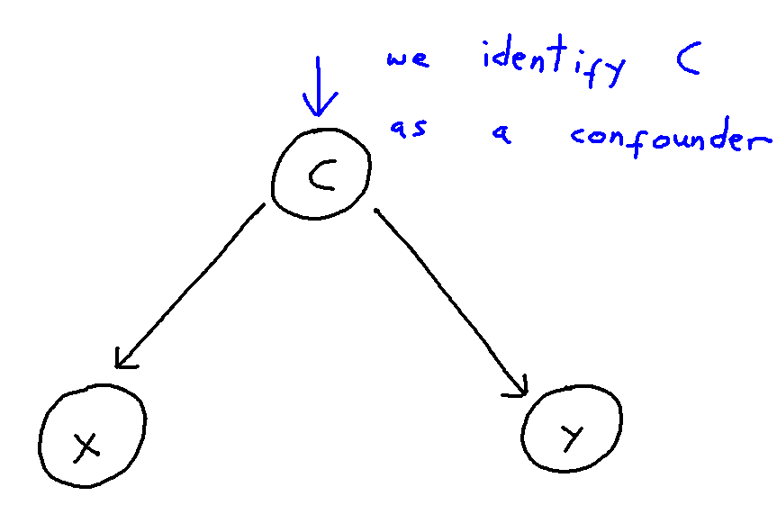
This problem can be though of in the following way:
We may control for a variable by means of including it within our regression or remove the influence of a variable altogether by stratifying our data. These, in turn, both remove the statistical association attributable to confounding. However, when the causal structure is larger and more complex, correctly handling confounding becomes trickier. Firstly, we risk inducing “selection”, and thus creating more confounding pathways, if we adjust for covariate which confounds the X-Y relationship but is itself also caused by other covariates. Secondly, if we adjust for an “instrument” of X, that being a covariate Z which is a cause of X but not of Y, then we risk amplifying bias from unseen confounding. Thirdly, further issues arise if many covariates within the model are correlated with each other, as then estimating a given causal effect becomes much more difficult, even for an unconfounded model.
Additionally, though this may seem to go without saying, we only have the variables that we have. Unmeasured confounding, from a covariate not within our dataset, can very much produce the same distortions but also be impossible to control for. With all this in mind, we look to the existing solutions to these above problems.
Solution: Confounder-Handling
There exist two broad solution types to the problem of confounder-handling, those being:
- A direct approach working from causal knowledge
- An indirect approach working from observed data
Existing knowledge-based solutions include:
- Back-door path criterion: [3]
- The back-door path criterion states that the causal effect is identifiable if there does not exist any “back door path” connecting the exposure X and outcome Y within the causal structure.
- As such, we may prevent confounding by controlling a variable present on any such existing path to “block” this path and thus prevent confounding via that path.
- Front-door path criterion: [3]
- The front-door path criterion states that the causal effect is identifiable (our statistical association is still a consistent estimator of the causal effect), even if the backdoor path criterion isn’t strictly satisfied. If we have a “mediator” covariate M, a covariate which sits between two covariates creating a direct path via itself, between X and Y, the the X-Y causal effect remains identifiable if we satisfy all of the following:
- M intercepts all causal pathways from X to Y
- There does not exist any backdoor path between X and M
- X blocks every backdoor path from M to Y
- The front-door path criterion states that the causal effect is identifiable (our statistical association is still a consistent estimator of the causal effect), even if the backdoor path criterion isn’t strictly satisfied. If we have a “mediator” covariate M, a covariate which sits between two covariates creating a direct path via itself, between X and Y, the the X-Y causal effect remains identifiable if we satisfy all of the following:
- Pre-treatment criterion: [4]
- The pre-treatment criterion states that, if we control for all covariates which occur prior to the exposure X in time, then we must necessarily have controlled for all confounders, and thus our causal effect is identifiable.
- Common-cause criterion : [4]
- The common-cause criterion states that, if we control for any and all covariates who mutually cause both the exposure X and outcome Y, then we must necessarily have controlled for all confounders.
- (Twice-modified) Disjunctive-cause criterion: [4]
- The (twice-modified) disjunctive cause criterion states that we can construct a sufficient adjustment set S in the following way:
- Add to our set S any pre-exposure covariate which is a cause of X, Y or both
- Remove from S any covariate Z which acts as an instrument of X
- Add to S any covariate which, though not satisfying condition 1, can act as a good proxy for unmeasured confounders of the X-Y relationship
- The (twice-modified) disjunctive cause criterion states that we can construct a sufficient adjustment set S in the following way:
- District criterion (iterative graph expansion): [5]
- The district criterion states that we have controlled for confounding if we our adjustment set S does indeed leave covariates X and Y in separate “districts” of a specially defined sub-graph of our wider causal structure, the setup of which is beyond the scope of this blog article.
- This criterion forms the theoretical justification to the method of iterative graph expansion proposed in the same paper, which readers are encouraged to find from the references if they would like to learn more.
Existing statistically-based solutions include:
- Step-wise regression: [6]
- Stepwise regression is a variable selection and model fitting procedure, which works by means of iteratively adding and removing explanatory variables (covariates other than X and Y) to form an optimal model where all explanatory variables are considered significant by some outside significance criterion (such as AIC).
- LASSO (Least absolute shrinkage and selection operator): [7]
- LASSO is a parameter estimation procedure typically employed for variable selection, which can be employed similarly for confounder identification.
More bespoke statistical solutions include:
- Change-in-estimate approach: [8]
- The change in estimate approach detects confounding via statistical significance testing, iteratively as covariates are added and removed. The idea, intuitively, is that if removing an outside variable as explanatory has a significant impact on the X-Y relationship, then it was likely confounding the two, and is identified as such.
- Targeted maximum likelihood estimators: [9]
- Targeted maximum likelihood estimators (TMLEs) are doubly-robust parameter estimators, which can be used for determining regression coefficients for statistical models while optimizing the bias-variance trade-off. This is used for confounder identification similarly to LASSO.
We have seen many approaches to the problem, but which is best? In thinking this through, we conclude that which approach is best depends on one’s intended use case. Specifically:
- Whether or not causal knowledge is available, with causal methods preferred as these provide guarantees of unconfoundedness in the result
- If causal knowledge is available, how much? Are we able to fully enumerate our problem?
Since different knowledge-based methods require different amounts of causal knowledge and provide stronger and weaker results correspondingly, it makes sense to select the approach most suited to the DAG we’re presently examining. However, knowledge-based methods scale poorly to larger causal structures, both in terms of running their algorithms and of enumerating the DAG to begin with – they quickly become intractable. Hence – statistical approaches, which provide weaker results with regards to unconfoundedness, but scale much better to larger causal scenarios and in principle require no causal knowledge to execute.
Conclusion
In conclusion, there exists a problem of confounding within the field of causal inference, and different solutions to this problem offer different advantages and disadvantages. Which solution is necessarily “best” depends upon your use case, specifically size of use-case and amount of causal knowledge available.
Contact Details
Miss Emma Jane Tarmey (she/her), University of Bristol, emma.tarmey@bristol.ac.uk
References
- Smith, George Davey and Phillips, Andrew N. Confounding in epidemiological studies: why ”independent” effects may not be all they seem. British Medical Journal, 305(6856):757–759, September 1992.
- Rothman, Kenneth J. et al. Serum Beta-Carotene: A Mechanism or ”Yellow Finger”? Epidemiology, 3(4):277–279, July 1992.
- Pearl, Judea. Causal diagrams for empirical research. Biometrika, 82(4):669–710, 1995.
- VanderWeele, Tyler J. Principles of Confounder Selection. European Journal of Epidemiology, 34:211–219, 2019, Section 4
- F. Richard Guo and Qingyuan Zhao. Confounder Selection via Iterative Graph Expansion. arXiv, October 2023
- VanderWeele, Tyler J. Principles of Confounder Selection. European Journal of Epidemiology, 34:211–219, 2019, Section 5
- Susan M. Shortreed and Ashkan Ertefaie. Outcome-Adaptive Lasso: Variable Selection for Causal Inference. Biometrics, 73:1111–1122, 2017. Publisher: Wiley.
- Talbot, Denis and Diop, Awa and Lavigne-Robichaud, Mathilde and Brisson, Chantal. The change in estimate method for selecting confounders: A simulation study. Statistical Methods in Medical Research 30(9):2032–2044, 2021.
- Schuler, Megan S. and Rose, Sherri. Targeted Maximum Likelihood Estimation for Causal Inference in Observational Studies. American Journal of Epidemiology, 185(1):65–73, January 2017.
Student Perspectives: Are larger models always better?
A post by Emma Ceccherini, PhD student on the Compass programme.
In December 2023, I attended NeurIPS, a machine learning conference, with some COMPASS colleagues. There, I attended a tutorial titled “Reconsidering Overfitting in the Age of Overparameterized Models”. The findings the speakers presented overturn some traditional statistical concepts, so I’d like to share some of these innovative ideas with the COMPASS blog readers.
Classical statistician vs deep learning practitioners
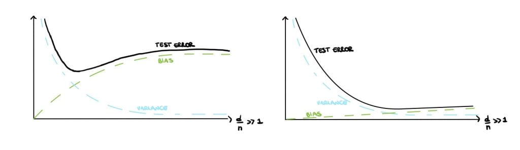
Classical statisticians argue that small models have high bias but large variance (Figure 1 (left)) and large models have low bias but high variance (Figure 1 (right)). This is called the bias-variance trade-off and is a crucial notion that can be found in all traditional statistic textbooks. Large, over-parameterised models perfectly interpolate the data points by fitting noise and they have a near-zero training error, but an increasing test error. This phenomenon is called overfitting and causes poor performances on unseen data. Overfitting implies low generalisation, which can be thought of as the model’s performance on newly generated data at test time.
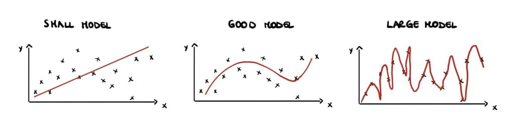
Therefore, statistics textbooks recommend avoiding overfitting and improving generalization by finding a balance in the bias-variance trade-off, either by reducing the number of parameters or using regularisation (Figure 1 (centre)).
However, as available computational power has increased, practitioners have made larger and larger models. For example, neural networks have millions of parameters, more than enough to fit noise, but they generalize very well in practice, performing significantly better than small models. These large over-parametrised models exceed the so-called interpolation threshold that is when the training error is approximately zero. Several theoretical statisticians are trying to infer what happens after this threshold. While we now have some answers, many questions are still up for debate!
The double descent
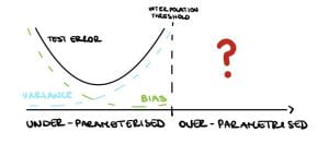
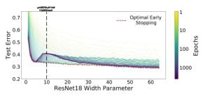
Nakkiran et al. [2019] show that in the under-parameterised regime, neural networks test errors exhibit the classical u-shape from the bias-variance trade-off, while in the over-parameterised regime, after the interpolation threshold, the test error decreases again creating the so-called double descent (see Figure 3). Figure 4 shows the test error of a neural network classifier on CIFAR-10, a standard image data set. The plot shows a double descent in the test error for neural networks trained until convergence (purple line).
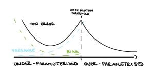
The authors make two more innovative observations: harmless interpolation and good generalisation for large models. It can be observed from Figure 4 that regularisation, equivalent to early stopping (red line), is substantially beneficial around the interpolation threshold. However, as the model size grows the test error for optimal early stopped neural networks (red line) and the one of neural networks trained until convergence test (purple line) overlap. Therefore, For large models, interpolation (trained until convergence) is not worse than regularisation (optimal early stopped), that is interpolation is harmless. Finally, Figure 4 shows that the test error is low as the size of the model grows. Hence, for large models, we can achieve reasonably good test accuracy, namely as a result of good generalisation.
Given these groundbreaking experimental results, statisticians seek to use theoretical analysis to understand when these three phenomena occur. Although neural networks were the initial motivation of this work, they are hard to analyse even for shallow networks. And so statisticians resorted to understanding these phenomena starting from the well-known linear models.
Over-parameterisation in linear models of the form $\mathbf{Y} = \mathbf{X}\theta^* + \mathbf{W}$ means there are more features $d$ than number of samples $n$, i.e. $d >n$ for an input matrix $\mathbf{X}$ of dimension $n \times d$. Then the system $\mathbf{X}\hat{\theta} = \mathbf{Y}$ has infinite solutions, thus consider the solution with minimum norm $\hat{\theta} = \text{arg min}||\hat{\theta}||_2$.
After the interpolation threshold, the variance is dominating (see Figure 3) so it needs to go down for the test error to go down. Indeed, Bartlett et al. [2020] show that in this setup the variance decreases as $d \gg n$, precisely $$\text{variance} \asymp \frac{\sigma^2n}{d}. $$
It can be shown that data is approximately orthogonal when $d \gg n$, namely $<X_i, X_j> \approx 0$ for $i \neq 0$, so the noise “energy” is spread out along the $d$ dimensions, hence as $d$ grows the noise contribution decreases.
However, Bartlett et al. [2020] also show that the bias increases with $d$, precisely $$\text{bias} \asymp (1-\frac{n}{d})||\theta^*||_2^2.$$ This is because the signal “energy” as well is spread out along $d$ dimensions.
Eventually, the bias will dominate and the test error will increase again, see Figure 5 (left). Therefore under this framework, the double descent and harmless interpolation can be achieved but good generalisation cannot.
Finally, Bartlett et al. [2020] show that in the special case where the $k$ features are “upweighted”, all three phenomena are observed. Assuming a spiked covariance $$\Sigma = \mathbb{E}[\mathbf{X}\mathbf{X}^T] = \begin{bmatrix}
R\mathbf{I}_k & \mathbf{0} \\
\mathbf{0} & \mathbf{I}_{d-k}
\end{bmatrix},$$ it can be shown that the variance and the bias will go to zero as $d \rightarrow \infty$ provided that $R \gg \frac{d}{n}$, therefore the double descent, harmless interpolation and good generalization are achieved (see Figure 5 (right)).
Many unanswered questions remain
Similar results to the ones described for linear models have been obtained for linear classification [Muthukumar et al., 2021]. While these types of results for neural networks [Frei et al., 2022] are still limited. Moreover, there are still many open questions on benign overfitting for neural networks. For example, the existing result focuses on $d \gg n$ regimes for neural networks, but there are no results on neural networks over-parameterised in low dimensions by increasing their width. Theoretical statisticians still have plenty of work to do to fully understand these phenomena!
References
Peter L. Bartlett, Philip M. Long, G´abor Lugosi, and Alexander Tsigler. Benign overfitting in linear
regression. Proceedings of the National Academy of Sciences, 117(48):30063–30070, April 2020. ISSN
1091-6490. doi: 10.1073/pnas.1907378117. URL http://dx.doi.org/10.1073/pnas.1907378117.
Spencer Frei, Gal Vardi, Peter L. Bartlett, Nathan Srebro, and Wei Hu. Implicit bias in leaky relu
networks trained on high-dimensional data, 2022.
Vidya Muthukumar, Adhyyan Narang, Vignesh Subramanian, Mikhail Belkin, Daniel Hsu, and Anant
Sahai. Classification vs regression in overparameterized regimes: Does the loss function matter?,
2021.
Preetum Nakkiran, Gal Kaplun, Yamini Bansal, Tristan Yang, Boaz Barak, and Ilya Sutskever. Deep
double descent: Where bigger models and more data hurt, 2019.
Compass students at ICLR 2024
Congratulations to Compass students Edward Milsom and Ben Anson who, along with their supervisor, had their paper accepted for a poster at ICLR 2024.
Convolutional Deep Kernel Machines
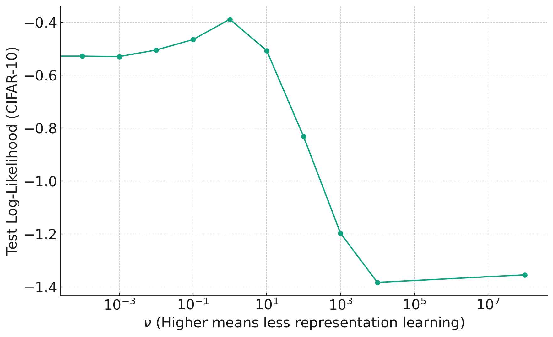
Ed and Ben: In this paper we explore the importance of representation learning in convolutional neural networks, specifically in the context of an infinite-width limit called the Neural Network Gaussian Process (NNGP) that is often used by theorists. Representation learning refers to the ability of models to learn a transformation of the data that is tailored to the task at hand. This is in contrast to algorithms that use a fixed transformation of the data, e.g. a support vector machine with a fixed kernel function like the RBF kernel. Representation learning is thought to be critical to the success of convolutional neural networks in vision tasks, but networks in the NNGP limit do not perform representation learning, instead transforming the data with a fixed kernel function. A recent modification to the NNGP limit, called the Deep Kernel Machine (DKM), allows one to gradually “add representation learning back in” to the NNGP, using a single hyperparameter that controls the amount of flexibility in the kernel. We extend this algorithm to convolutional architectures, which required us to develop a new sparse inducing point approximation scheme. This allowed us to test on the full CIFAR-10 image classification dataset, where we achieved state-of-the-art test accuracy for kernel methods, with 92.7%.
In the plot below, we see how changing the hyperparameter (x-axis) to reduce flexibility too much harms the performance on unseen data.
Student Perspectives: Group Testing
A post by Rahil Morjaria, PhD student on the Compass programme.
What is Group Testing?
Group Testing was first introduced in the 1940s as a way to test military recruits for syphilis during World War II. By combining blood samples, they hoped to reduce the total number of tests needed to detect the diseased individuals (compared to testing each recruit individually).
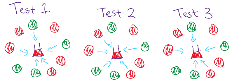
Example of pooling blood samples, where red and green depicts diseased and not diseased respectively.
Since then, there have been many advances in Group Testing with applications not just in detecting diseased individuals but also in communications, cybersecurity and data storage. In essence, whenever we have a situation where we need to detect a proportionally rare occurrence, Group Testing is probably applicable.
More formally, if we have some diseased set of individuals of size $k$ of a total population $n$, it might be considered (instead of testing each individual separately) to pool people together into groups (with replacement) and test these groups.
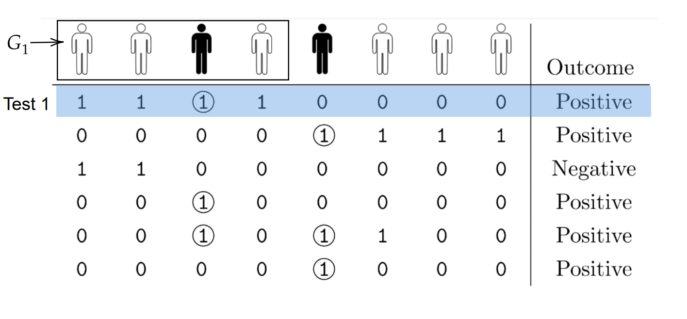
Matrix Form of Group Testing (each row depicting a test and each column depicting a member of the population) [1].
We often write our test design in matrix form where each row is a group/test and each column indicates a member of the population, where a $1$ indicates a individuals inclusion in a test.
The relationship between $k$ and $n$ is quite important, our focus is on the sparse case in which $k = O(n^\alpha)$ where $\alpha \in (0,1)$.
Often we assume our test apparatus is sensitive enough where a single diseased individual in the test will give us a positive result (as shown in the image above) this is known as the noiseless case (there is vast amounts of work done for different types of noise, for more information check out [1]).
Adaptive vs Non-Adaptive Group Testing
Adaptive Group Testing (as the name suggests) allows us to adapt our subsequent tests by the results of the previous. If we compare this to Non-Adaptive Group Testing, in which we have to define our tests (and thus our groups) before we obtain any results, we can expect stronger results.
As our tests have binary outputs, we can obtain at most $1$ bit of information per test. As there are $\binom{n}{k}$ possible defective sets, we would need $\log_2\binom{n}{k}$ bits to uniquely represent each possible set. This gives us the limit of $\log_2\binom{n}{k}$ tests needed, this is known as a converse result, a fundamental limit which we are unable to overcome.
In the noiseless case, Adaptive Group Testing is able to achieve this fundamental limit. First we split our total items $n$ into $k$ (the number of defective items) subsets of length $n/k$ without replacement, and then perform Binary Splitting.
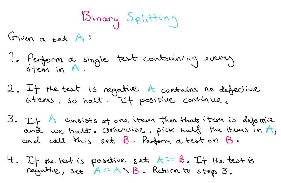
Binary Splitting Adaptive Algorithm.
While Adaptive Group Testing is able to reach fundamental limits, our main focus is on Non-Adaptive Group Testing. Non-Adaptive Group Testing has many applications due to it’s ability to be ran in parallel (and other ease of use situations).
Non-Adaptive Group Testing procedures are often designed randomly (in which each items inclusion in a test is $Bern(v)$ for some $v$) or with near constant column weight (each item is in ‘nearly’ the same amount of tests). Out of these 2 designs near constant column weight gives stronger results.
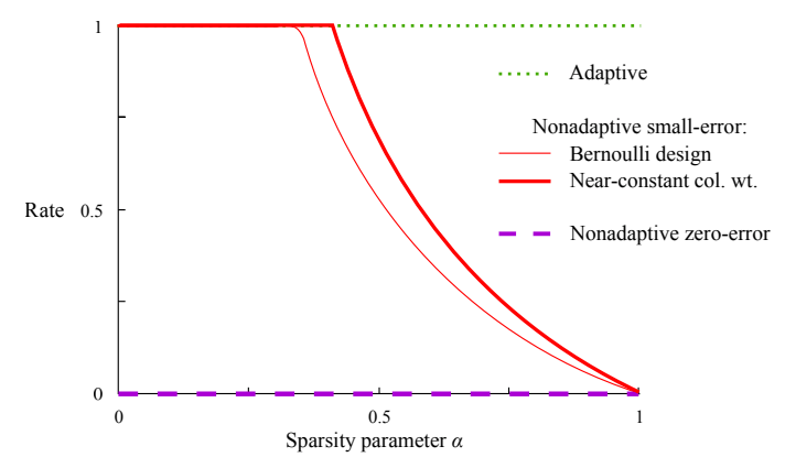 A graph comparing different group testing designs, where the $\text{Rate} = \log_2\binom{n}{k}/T$ where $T$ is the number of tests needed to recover all the defective items (with high probability for the red lines and with certainty for the purple line). [1]
Goals
While there are many strong results in Group Testing, there is still much to explore. From looking at List Decoding (in which we allow a list of possible defective sets to be outputted), other forms of noise and our efficient algorithms still not being able to match up to our theoretical achievable methods, there is work to be done in all aspects. With improvements in technology, combined with the myriad of applications, the future of Group Testing definitely looks bright!
References:
[1] M. Aldridge, O. Johnson, and J. Scarlett. Group testing: an information theory perspective. CoRR, abs/1902.06002, 2019. URL http://arxiv.org/abs/1902.06002.
Student Perspectives: SPREE Methods for Small Area Estimation
A post by Codie Wood, PhD student on the Compass programme.
This blog post is an introduction to structure preserving estimation (SPREE) methods. These methods form the foundation of my current work with the Office for National Statistics (ONS), where I am undertaking a six-month internship as part of my PhD. During this internship, I am focusing on the use of SPREE to provide small area estimates of population characteristic counts and proportions.
Small area estimation
Small area estimation (SAE) refers to the collection of methods used to produce accurate and precise population characteristic estimates for small population domains. Examples of domains may include low-level geographical areas, or population subgroups. An example of an SAE problem would be estimating the national population breakdown in small geographical areas by ethnic group [2015_Luna].
Demographic surveys with a large enough scale to provide high-quality direct estimates at a fine-grain level are often expensive to conduct, and so smaller sample surveys are often conducted instead.
SAE methods work by drawing information from different data sources and similar population domains in order to obtain accurate and precise model-based estimates where sample counts are too small for high quality direct estimates. We use the term small area to refer to domains where we have little or no data available in our sample survey.
SAE methods are frequently relied upon for population characteristic estimation, particularly as there is an increasing demand for information about local populations in order to ensure correct allocation of resources and services across the nation.
Structure preserving estimation
Structure preserving estimation (SPREE) is one of the tools used within SAE to provide population composition estimates. We use the term composition here to refer to a population break down into a two-way contingency table containing positive count values. Here, we focus on the case where we have a population broken down into geographical areas (e.g. local authority) and some subgroup or category (e.g. ethnic group or age).
Orginal SPREE-type estimators, as proposed in [1980_Purcell], can be used in the case when we have a proxy data source for our target composition, containing information for the same set of areas and categories but that may not entirely accurately represent the variable of interest. This is usually because the data are outdated or have a slightly different variable definition than the target.
We also incorporate benchmark estimates of the row and column totals for our composition of interest, taken from trusted, quality assured data sources and treated as known values. This ensures consistency with higher level known population estimates. SPREE then adjusts the proxy data to the estimates of the row and column totals to obtain the improved estimate of the target composition.

An illustration of the data required to produce SPREE-type estimates.
In an extension of SPREE, known as generalised SPREE (GSPREE) [2004_Zhang], the proxy data can also be supplemented by sample survey data to generate estimates that are less subject to bias and uncertainty than it would be possible to generate from each source individually. The survey data used is assumed to be a valid measure of the target variable (i.e. it has the same definition and is not out of date), but due to small sample sizes may have a degree of uncertainty or bias for some cells.
The GSPREE method establishes a relationship between the proxy data and the survey data, with this relationship being used to adjust the proxy compositions towards the survey data.

An illustration of the data required to produce GSPREE estimates.
GSPREE is not the only extension to SPREE-type methods, but those are beyond the scope of this post. Further extensions such as Multivariate SPREE are discussed in detail in [2016_Luna].
Original SPREE methods
First, we describe original SPREE-type estimators. For these estimators, we require only well-established estimates of the margins of our target composition.
We will denote the target composition of interest by $\mathbf{Y} = (Y{aj})$, where $Y{aj}$ is the cell count for small area $a = 1,\dots,A$ and group $j = 1,\dots,J$. We can write $\mathbf Y$ in the form of a saturated log-linear model as the sum of four terms,
$$ \log Y_{aj} = \alpha_0^Y + \alpha_a^Y + \alpha_j^Y + \alpha_{aj}^Y.$$
There are multiple ways to write this parameterisation, and here we use the centered constraints parameterisation given by $$\alpha_0^Y = \frac{1}{AJ}\sum_a\sum_j\log Y_{aj},$$ $$\alpha_a^Y = \frac{1}{J}\sum_j\log Y_{aj} – \alpha_0^Y,$$ $$\alpha_j^Y = \frac{1}{A}\sum_a\log Y_{aj} – \alpha_0^Y,$$ $$\alpha_{aj}^Y = \log Y_{aj} – \alpha_0^Y – \alpha_a^Y – \alpha_j^Y,$$
which satisfy the constraints $\sum_a \alpha_a^Y = \sum_j \alpha_j^Y = \sum_a \alpha_{aj}^Y = \sum_j \alpha_{aj}^Y = 0.$
Using this expression, we can decompose $\mathbf Y$ into two structures:
- The association structure, consisting of the set of $AJ$ interaction terms $\alpha_{aj}^Y$ for $a = 1,\dots,A$ and $j = 1,\dots,J$. This determines the relationship between the rows (areas) and columns (groups).
- The allocation structure, consisting of the sets of terms $\alpha_0^Y, \alpha_a^Y,$ and $\alpha_j^Y$ for $a = 1,\dots,A$ and $j = 1,\dots,J$. This determines the size of the composition, and differences between the sets of rows (areas) and columns (groups).
Suppose we have a proxy composition $\mathbf X$ of the same dimensions as $\mathbf Y$, and we have the sets of row and column margins of $\mathbf Y$ denoted by $\mathbf Y_{a+} = (Y_{1+}, \dots, Y_{A+})$ and $\mathbf Y_{+j} = (Y_{+1}, \dots, Y_{+J})$, where $+$ substitutes the index being summed over.
We can then use iterative proportional fitting (IPF) to produce an estimate $\widehat{\mathbf Y}$ of $\mathbf Y$ that preserves the association structure observed in the proxy composition $\mathbf X$. The IPF procedure is as follows:
- Rescale the rows of $\mathbf X$ as $$ \widehat{Y}_{aj}^{(1)} = X_{aj} \frac{Y_{+j}}{X_{+j}},$$
- Rescale the columns of $\widehat{\mathbf Y}^{(1)}$ as $$ \widehat{Y}_{aj}^{(2)} = \widehat{Y}_{aj}^{(1)} \frac{Y_{a+}}{\widehat{Y}_{a+}^{(1)}},$$
- Rescale the rows of $\widehat{\mathbf Y}^{(2)}$ as $$ \widehat{Y}_{aj}^{(3)} = \widehat{Y}_{aj}^{(2)} \frac{Y_{+j}}{\widehat{Y}_{+j}^{(2)}}.$$
Steps 2 and 3 are then repeated until convergence occurs, and we have a final composition estimate denoted by $\widehat{\mathbf Y}^S$ which has the same association structure as our proxy composition, i.e. we have $\alpha_{aj}^X = \alpha_{aj}^Y$ for all $a \in \{1,\dots,A\}$ and $j \in \{1,\dots,J\}.$ This is a key assumption of the SPREE implementation, which in practise is often restrictive, motivating a generalisation of the method.
Generalised SPREE methods
If we can no longer assume that the proxy composition and target compositions have the same association structure, we instead use the GSPREE method first introduced in [2004_Zhang], and incorporate survey data into our estimation process.
The GSPREE method relaxes the assumption that $\alpha_{aj}^X = \alpha_{aj}^Y$ for all $a \in \{1,\dots,A\}$ and $j \in \{1,\dots,J\},$ instead imposing the structural assumption $\alpha_{aj}^Y = \beta \alpha_{aj}^X$, i.e. the association structure of the proxy and target compositions are proportional to one another. As such, we note that SPREE is a particular case of GSPREE where $\beta = 1$.
Continuing with our notation from the previous section, we proceed to estimate $\beta$ by modelling the relationship between our target and proxy compositions as a generalised linear structural model (GLSM) given by
$$\tau_{aj}^Y = \lambda_j + \beta \tau_{aj}^X,$$ with $\sum_j \lambda_j = 0$, and where $$ \begin{align} \tau_{aj}^Y &= \log Y_{aj} – \frac{1}{J}\sum_j\log Y_{aj},\\
&= \alpha_{aj}^Y + \alpha_j^Y,
\end{align}$$ and analogously for $\mathbf X$.
It is shown in [2016_Luna] that fitting this model is equivalent to fitting a Poisson generalised linear model to our cell counts, with a $\log$ link function. We use the association structure of our proxy data, as well as categorical variables representing the area and group of the cell, as our covariates. Then we have a model given by $$\log Y_{aj} = \gamma_a + \tilde{\lambda}_j + \tilde{\beta}\alpha_{aj}^X,$$ with $\gamma_a = \alpha_0^Y + \alpha_a^Y$, $\tilde\lambda_j = \alpha_j^Y$ and $\tilde\beta \alpha_{aj}^X = \alpha_{aj}^Y.$
When fitting the model we use survey data $\tilde{\mathbf Y}$ as our response variable, and are then able to obtain a set of unbenchmarked estimates of our target composition. The GSPREE method then benchmarks these to estimates of the row and column totals, following a procedure analagous to that undertaken in the orginal SPREE methodology, to provide a final set of estimates for our target composition.
ONS applications
The ONS has used GSPREE to provide population ethnicity composition estimates in intercensal years, where the detailed population estimates resulting from the census are outdated [2015_Luna]. In this case, the census data is considered the proxy data source. More recent works have also used GSPREE to estimate counts of households and dwellings in each tenure at the subnational level during intercensal years [2023_ONS].
My work with the ONS has focussed on extending the current workflows and systems in place to implement these methods in a reproducible manner, allowing them to be applied to a wider variety of scenarios with differing data availability.
References
[1980_Purcell] Purcell, Noel J., and Leslie Kish. 1980. ‘Postcensal Estimates for Local Areas (Or Domains)’. International Statistical Review / Revue Internationale de Statistique 48 (1): 3–18. https://doi.org/10/b96g3g.
[2004_Zhang] Zhang, Li-Chun, and Raymond L. Chambers. 2004. ‘Small Area Estimates for Cross-Classifications’. Journal of the Royal Statistical Society Series B: Statistical Methodology 66 (2): 479–96. https://doi.org/10/fq2ftt.
[2015_Luna] Luna Hernández, Ángela, Li-Chun Zhang, Alison Whitworth, and Kirsten Piller. 2015. ‘Small Area Estimates of the Population Distribution by Ethnic Group in England: A Proposal Using Structure Preserving Estimators’. Statistics in Transition New Series and Survey Methodology 16 (December). https://doi.org/10/gs49kq.
[2016_Luna] Luna Hernández, Ángela. 2016. ‘Multivariate Structure Preserving Estimation for Population Compositions’. PhD thesis, University of Southampton, School of Social Sciences. https://eprints.soton.ac.uk/404689/.
[2023_ONS] Office for National Statistics (ONS), released 17 May 2023, ONS website, article, Tenure estimates for households and dwellings, England: GSPREE compared with Census 2021 data
Student Perspectives: Semantic Search
A post by Ben Anson, PhD student on the Compass programme.
Semantic Search
Semantic search is here. We already see it in use in search engines [13], but what is it exactly and how does it work?
Search is about retrieving information from a corpus, based on some query. You are probably using search technology all the time, maybe $\verb|ctrl+f|$, or searching on google. Historically, keyword search, which works by comparing the occurrences of keywords between queries and documents in the corpus, has been surprisingly effective. Unfortunately, keywords are inherently restrictive – if you don’t know the right one to use then you are stuck.
Semantic search is about giving search a different interface. Semantic search queries are provided in the most natural interface for humans: natural language. A semantic search algorithm will ideally be able to point you to a relevant result, even if you only provided the gist of your desires, and even if you didn’t provide relevant keywords.

Figure 1 illustrates a concrete example where semantic search might be desirable. The query ‘animal’ should return both the dog and cat documents, but because the keyword ‘animal’ is not present in the cat document, the keyword model fails. In other words, keyword search is susceptible to false negatives.
Transformer neural networks turn out to be very effective for semantic search [1,2,3,10]. In this blog post, I hope to elucidate how transformers are tuned for semantic search, and will briefly touch on extensions and scaling.
The search problem, more formally
Suppose we have a big corpus $\mathcal{D}$ of documents (e.g. every document on wikipedia). A user sends us a query $q$, and we want to point them to the most relevant document $d^*$. If we denote the relevance of a document $d$ to $q$ as $\text{score}(q, d)$, the top search result should simply be the document with the highest score,
$$
d^* = \mathrm{argmax}_{d\in\mathcal{D}}\, \text{score}(q, d).
$$
This framework is simple and it generalizes. For $\verb|ctrl+f|$, let $\mathcal{D}$ be the set of individual words in a file, and $\text{score}(q, d) = 1$ if $q=d$ and $0$ otherwise. The venerable keyword search algorithm BM25 [4], which was state of the art for decades [8], uses this score function.
For semantic search, the score function is often set as the inner product between query and document embeddings: $\text{score}(q, d) = \langle \phi(q), \phi(d) \rangle$. Assuming this score function actually works well for finding relevant documents, and we use a simple inner product, it is clear that the secret sauce lies in the embedding function $\phi$.
Transformer embeddings
We said above that a common score function for semantic search is $\text{score}(q, d) = \langle \phi(q), \phi(d) \rangle$. This raises two questions:
- Question 1: what should the inner product be? For semantic search, people tend to use the cosine similarity for their inner product.
- Question 2: what should $\phi$ be? The secret sauce is to use a transformer encoder, which is explained below.
Quick version
Transformers magically gives us a tunable embedding function $\phi: \text{“set of all pieces of text”} \rightarrow \mathbb{R}^{d_{\text{model}}}$, where $d_{\text{model}}$ is the embedding dimension.
More detailed version
See Figure 2 for an illustration of how a transformer encoder calculates an embedding for a piece of text. In the figure we show how to encode “cat”, but we can encode arbitrary pieces of text in a similar way. The transformer block details are out of scope here; though, for these details I personally found Attention is All You Need [9] helpful, the crucial part being the Multi-Head Attention which allows modelling dependencies between words.
Figure 2: Transformer illustration (transformer block image taken from [6])
The transformer encoder is very flexible, with almost every component parameterized by a learnable weight / bias – this is why it can be used to model the complicated semantics in natural language. The pooling step in Figure 2, where we map our sequence embedding $X’$ to a fixed size, is not part of a ‘regular’ transformer, but it is essential for us. It ensures that our score function $\langle \phi(q), \phi(d) \rangle$ will work when $q$ and $d$ have different sizes.
Making the score function good for search
There is a massive issue with transformer embedding as described above, at least for our purposes – there is no reason to believe it will satisfy simple semantic properties, such as,
$\text{score}(\text{“busy place”}, \text{“tokyo”}) > \text{score}(\text{“busy place”}, \text{“a small village”})$
‘But why would the above not work?’ Because, of course, transformers are typically trained to predict the next token in a sequence, not to differentiate pieces of text according to their semantics.
The solution to this problem is not to eschew transformer embeddings, but rather to fine-tune them for search. The idea is to encourage the transformer to give us embeddings that place semantically dissimilar items far apart. E.g. let $q=$’busy place’, then we want $ d^+=$’tokyo’ to be close to $q$ and $d^-=$’a small village’ to be far away.
This semantic separation can be achieved by fine-tuning with a contrastive loss [1,2,3,10],
$$
\text{maximize}_{\theta}\,\mathcal{L} = \log \frac{\exp(\text{score}(q, d^+))}{\exp(\text{score}(q, d^+)) + \exp(\text{score}(q, d^-))},
$$
where $\theta$ represents the transformer parameters. The $\exp$’s in the contastive loss are to ensure we never divide by zero. Note that we can interpret the contrastive loss as doing classification since we can think of the argument to the logarithm as $p(d^+ | q)$.
That’s all we need, in principle, to turn a transformer encoder into a text embedder! In practice, the contrastive loss can be generalized to include more positive and negative examples, and it is indeed a good idea to have a large batch size [11] (intuitively it makes the separation of positive and negative examples more difficult, resulting in a better classifier). We also need a fine-tuning dataset – a dataset of positive/negative examples. OpenAI showed that it is possible to construct one in an unsupervised fashion [1]. However, there are also publicly available datasets for supervised fine-tuning, e.g. MSMARCO [12].
Extensions
One really interesting avenue of research is training of general purposes encoders. The idea is to provide instructions alongside the queries/documents [2,3]. The instruction could be $\verb|Embed this document for search: {document}|$ (for the application we’ve been discussing), or $\verb|Embed this document for clustering: {document}|$ to get embeddings suitable for clustering, or $\verb|Embed this document for sentiment analysis: {document}|$ for embeddings suitable for sentiment analysis. The system is fine-tuned end-to-end with the appropriate task, e.g. a contrastive learning objective for the search instruction, a classification objective for sentiment analysis, etc., leaving us with an easy way to generate embeddings for different tasks.
A note on scaling
The real power of semantic (and keyword) search comes when a search corpus is too large for a human to search manually. However if the corpus is enormous, we’d rather avoid looking at every document each time we get a query. Thankfully, there are methods to avoid this by using specially tailored data structures: see Inverted Indices for keyword algorithms, and Hierarchical Navigable Small World graphs [5] for semantic algorithms. These both reduce search time complexity from $\mathcal{O}(|\mathcal{D}|)$ to $\mathcal{O}(\log |\mathcal{D}|)$, where $|\mathcal{D}|$ is the corpus size.
There are many startups (Pinecone, Weviate, Milvus, Chroma, etc.) that are proposing so-called vector databases – databases in which embeddings are stored, and queries can be efficiently performed. Though, there is also work contesting the need for these types of database in the first place [7].
Summary
We summarised search, semantic search, and how transformers are fine-tuned for search with a contrastive loss. I personally find this a very nice area of research with exciting real-world applications – please reach out (ben.anson@bristol.ac.uk) if you’d like to discuss it!
References
[1]: Text and code embeddings by contrastive pre-training, Neelakantan et al (2022)
[2]: Task-aware Retrieval with Instructions, Asai et al (2022)
[3]: One embedder, any task: Instruction-finetuned text embeddings, Su et al (2022)
[4]: Some simple effective approximations to the 2-poisson model for probabilistic weighted retrieval, Robertson and Walker (1994)
[5]: Efficient and robust approximate nearest neighbor search using Hierarchical Navigable Small World graphs, https://arxiv.org/abs/1603.09320
[6]: An Image is Worth 16×16 Words: Transformers for Image Recognition at Scale, https://arxiv.org/abs/2010.11929
[7]: Vector Search with OpenAI Embeddings: Lucene Is All You Need, arXiv preprint arXiv:2308.14963
[8]: Complement lexical retrieval model with semantic residual embeddings, Advances in Information Retrieval (2021)
[9]: Attention is all you need, Advances in neural information processing systems (2017)
[10]: Sgpt: Gpt sentence embeddings for semantic search, arXiv preprint arXiv:2202.08904
[11]: Contrastive representation learning: A framework and review, IEEE Access 8 (2020)
[12]: Ms marco: A human generated machine reading comprehension dataset, arXiv preprint arXiv:1611.09268
[13]: AdANNS: A Framework for Adaptive Semantic Search, arXiv preprint arXiv:2305.19435
Student Perspectives: Machine Learning Models for Probability Distributions
A post by Tennessee Hickling, PhD student on the Compass programme.
Introduction
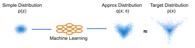
Probabilistic modelling provides a consistent way to deal with uncertainty in data. The central tool in this methodology is the probability distribution, which describes the randomness of observations. To create effective models of reality, we need to be able to specify probability distributions that are flexible enough to capture real phenomena whilst remaining feasible to estimate. In the past decade machine learning (ML) has developed many new and exciting ways to represent and learn potentially complex probability distributions.
ML has provided significant advances in modelling of high dimensional and highly structured data such as images or text. Many of these modern approaches are applied as “generative models”. The goal of such approaches is to sample new synthetic observations from an approximate distribution which closely matches the target distribution. For example, we may use many images of cats to learn an approximate distribution, from which we can sample new images of cats that appear realistic. Usually, a “generative model” indicates the requirement to sample from the model, but not necessarily assign probabilities to observed data. In this case, the model captures uncertainty by imitating the structure and randomness of the data.
Many of these modern methods work by transforming simple randomness (such as a Normal distribution) into the target complex randomness. In my own research, I work on a known limitation of such approaches to replicate a particular aspect of randomness – the tails of probability distributions [1, 11]. In this post, I wanted to take a step back and provide an overview of and connections between two ML methods that can be used to model probability distributions – Normalising Flows (NFs) and Variational Autoencoders (VAEs).
Figure 1: Basic illustration of ML learning of a distribution. We optimise the machine learning model to produce a distribution close to our target. This is often conceptualised in the generative direction, such that our ML model moves samples from the simple distribution to more closely match the target observations.
Some Background
Consider real valued vectors $z \in \mathbb{R}^{d_z}$ and $x \in \mathbb{R}^{d_x}$. In this post I mirror notation used in [2], where $p(x)$ refers to the density and distribution of $x$ and $x \sim p(x)$ indicates samples according to that distribution. The generic set up I am considering is that of density estimation – trying to model the distribution $p(x)$ of some observed data $\{x_i\}_{i=1}^{N}$. I use a semicolon to denote parameters, so $p(x; \beta)$ is a distribution over $x$ with parameters $\beta$. I also make use of different letters to distinguish different distributions, for example using $q(x)$ to denote an approximation to $p(x)$. The notation $\mathbb{E}_p[f(x)]$ refers to the standard expectation of $f(x)$ over the distribution $p$.
The discussed methods introduce some simple source of randomness arising from a known, simple latent distribution $p(z)$. This is also referred to in some literature as the prior, though the usage is not straightforwardly relatable to traditional Bayesian concepts. The goal is then to fit an approximate $q(x|z; \theta)$, that is a conditional distribution, such that $$q(x; \theta) = \int q(x|z; \theta)p(z)dz \approx p(x),$$in words, the marginal density over $x$ implied by the conditional density, is close to our target distribution $p(x)$. In general, we can’t compute $q(x)$, as we can’t solve the above integral for very flexible $q(x | z; \theta)$.
Variational Inference
We commonly make use of the Kullback-Leibler (KL) divergence, which can be interpreted as measuring the difference between two probability distributions. It is a useful practical tool, since we can compute and optimise the quantity in a wide variety of situations. Techniques which optimise a probability distribution using such divergences are known as variational methods. There are other choices of divergence, but KL is the most standard. Important properties of KL are that the quantity $KL(p|| q)$ is non-negative and non-symmetric i.e. $KL(p|| q) \neq KL(q || p)$.
Given this, we can see that a natural objective is to minimise the difference between distributions, as measured by the KL, $$KL(p(x) || q(x; \theta)) = \int p(x) \log \frac{p(x)}{q(x; \theta)} dx.$$Advances in this area have mostly developed new ways to make this optimisation tractable for flexible $q(x | z; \theta)$.
Normalising Flow
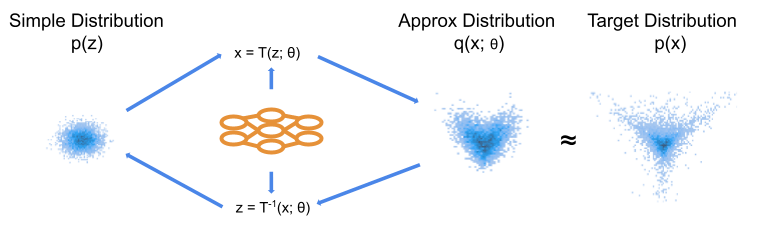
A normalising flow is a parameterised transformation of a random variable. The key simplifying assumption is that the forward generation is deterministic. That is, for $d_x = d_z$, that $$
x = T(z; \theta),$$for some transformation function $T$. We additionally require that $T$ is a differentiable bijection. Given these requirements, we can express the approximate density of $x$ exactly as $$q_x(x; \theta) = p_z(T^{-1}(x; \theta))\big|\text{det } J_{T^{-1}}(x; \theta)\big|.$$Here, $\text{det }J_{T^{-1}}$ is the determinant of the Jacobian of the inverse transformation. Research on NFs has developed numerous ways to make the computation of the Jacobian term tractable. The standard approach is to use neural networks to produce $\theta$ (the parameters of the transformation), with numerous ways of configuring the model to capture dependency between dimensions. Additionally, we often stack many layers to provide more flexibility. See [10] and the review [2] for more details on how this is achieved.
As we have access to an analytic approximate density, we can minimise the negative log-likelihood of our model, $$\mathcal{J}(\theta) = -\sum_{i=1}^{N} \log q(x_i; \theta),$$which is the Monte-Carlo approximation of the KL loss (up to an additive constant). This is straightforward to optimise using stochastic gradient descent [9] and automatic differentiation.
Figure 2: Schematic of NF model. The ML model produces the parameters of our transformation, which are identical in the forward and backwards directions. We choose the transformation such that we can express an analytic density function for our approximate distribution.
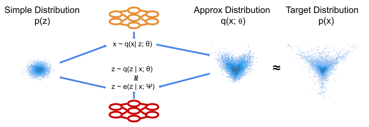
Variational Autoencoder
In the Variational Autoencoder (VAE) [3] the conditional distribution $q(x| z; \theta)$ is known as the decoder. VAEs consider the marginal in terms of the posterior, that is $$q(x; \theta) = \frac{q(x | z; \theta)p(z)}{q(z | x; \theta)}.$$The posterior $q(z | x; \theta)$ is itself not generally tractable. VAEs proceed by introducing an encoder, which approximates $q(z | x; \theta)$. This is itself simply a conditional distribution $e(z | x; \psi)$. We use this approximation to express the log marginal over $x$ as below.
$$\begin{align}
\log q(x; \theta) &= \mathbb{E}_{e}\bigg[\log q(x; \theta)\frac{e(z | x; \psi)}{e(z | x; \psi)}\bigg] \\
&= \mathbb{E}_{e}\bigg[\log\frac{q(x | z; \theta)p(z)}{q(z | x; \theta)}\frac{e(z | x; \psi)}{e(z | x; \psi)}\bigg] \\
&= \mathbb{E}_{e}\bigg[\log\frac{q(x | z; \theta)p(z)}{e(z | x; \psi)}\bigg] + KL(e(z | x; \psi) || q(z | x; \theta)) \\
&= \mathcal{J}_{\theta,\psi} + KL(e(z | x; \psi) || q(z | x; \theta))
\end{align}$$
The additional approximation gives a more complex expression and does not provide an analytical approximate density. However, as $KL(e(z | x; \psi) || q(z | x; \theta))$ is positive, $\mathcal{J}_{\theta,\psi}$ forms a lower bound on $\log q(x; \theta)$. This expression is commonly referred to as the Evidence Lower Bound (or ELBO). The second term, the divergence between our encoder and the implied posterior will be minimised as we increase $\mathcal{J}_{\theta,\psi}$ in $\psi$. As we increase $\mathcal{J}_{\theta,\psi}$, we will either be increasing $\log q(x; \theta)$ or reducing $KL(e(z | x; \psi) || q(z | x; \theta))$.
The goal is to increase $\log q(x; \theta)$, which we hope occurs as we optimise over both parameters. This ambiguity in optimisation results in well known issues, such as posterior collapse [12] and can result in some counter-intuitive behaviour [4]. Despite this, VAEs remain a powerful and popular approach. An important benefit is that we no longer require $d_x = d_z$, which means we can map high dimensional $x$ to low dimensional $z$ to perform dimensionality reduction.
Figure 3: Schematic of VAE model. We now have a stochastic forward transformation. To optimise this we introduce a decoder model which approximates the posterior implied by the forward transformation. We now have a more flexible transformation, but two models to train and no analytic approximate density.
Surjective Flows
We can now identify a connection between NFs and VAEs. Recent work has reinterpreted NFs within the VAE framework, permitting a broader class of transitions whilst retaining analytic tractability of NFs [5]. Considering our decoding conditional as $$q(x|z; \theta) = \delta(x – T(z; \theta)),$$ we have the posterior exactly as
$$q(z|x; \theta) = \delta(z – T^{-1}(x; \theta)),$$
where $\delta$ is the dirac delta function.
This provides a view of a NF as a special case of a VAE, where we don’t need to approximate the posterior. Considering our VAE approximation, $$
\log q(x; \theta) = \mathbb{E}_e\big[\log p(z) + \log\frac{q(x | z; \theta)}{e(z | x; \psi)}\big] + KL(e(z | x; \psi) || q(z | x; \theta)),
$$and taking $e(z | x; \psi) = q(z | x; \theta)$, then the final KL term is 0 by definition. In that case, we recover our analytic density for NFs (see [5] for details).
Note that accessing an analytic density depends on having $e(z | x; \psi) = q(z | x; \theta)$ and computing $$\mathbb{E}_e\big[\log p(z) + \log\frac{q(x | z; \theta)}{e(z | x; \psi)}\big].$$These requirements are actually weaker than those we apply in the case of standard NFs. Consider a deterministic transformation $T^{-1}(x)$ which is surjective, crucially we can have many $x$ which map to the same $z$, so no longer have an analytic inverse. However we can still choose a $q(x | z)$ which is stochastic inverse of $T^{-1}$. For example, consider an absolute value surjection, $q(z | x) = \delta(z – |x|)$, to invert this transformation we can choose $q(x | z) = \frac{1}{2}\delta(x – z) + \frac{1}{2}\delta(x + z)$, which we can sample from straight-forwardly. This transformation enforces symmetry across the origin in the approximate distribution, a potentially useful inductive bias. In this example, and many others, we can also compute the density exactly. This has led to a number of interesting extensions to NFs, such as “funnel flows” which have $d_z < d_x$ but retain an analytic approximate density [6]. As we retain an analytic approximate density, we can optimise them in the same way as NFs.
Figure 4: Schematic of a surjective transformation. We have a stochastic forward transformation, but the inverse is deterministic. This restricts what transformations we can have, but retains an analytic approximate density.

Conclusion
I have presented an overview of two widely-used methods for modelling probability distributions with machine learning techniques. I’ve also highlighted an interesting connection between these methods, an area of research that has led to the development of interesting new models. It’s worth noting that other important classes of ML models such as Generative Adversarial Networks and Diffusion models can also be interpreted as approximate probability distributions. There are many superficial connections between those methods and the ones discussed here. Exploring these theoretical similarities presents an compelling direction of research to sharpen understanding of such models’ relative advantages. Another promising direction is the synthesis of these methods, where researchers aim to harness the strengths of each approach [7,8]. This not only enhances the existing knowledge base but also offers opportunities for innovative applications in the field.
References
[1] Jaini, Priyank, et al. “Tails of Lipschitz triangular flows.” International Conference on Machine Learning. PMLR, 2020
[2] Papamakarios, G., et al. “Normalizing flows for probabilistic modeling and inference.” Journal of Machine Learning Research, 2021
[3] Kingma, Diederik P., and Max Welling. “Auto-encoding variational bayes.” arXiv:1312.6114, 2013
[4] Rainforth, Tom, et al. “Tighter variational bounds are not necessarily better.” International Conference on Machine Learning. PMLR, 2018
[5] Nielsen, Didrik, et al. “Survae flows: Surjections to bridge the gap between vaes and flows.” Advances in Neural Information Processing, 2020
[6] Samuel Klein, et al. “Funnels: Exact maximum likelihood with dimensionality reduction.” arXiv:2112.08069, 2021
[7] Kingma, Durk P., et al. “Improved variational inference with inverse autoregressive flow.” Advances in neural information processing systems , 2016
[8] Zhang, Qinsheng, and Yongxin Chen. “Diffusion normalizing flow.” Advances in Neural Information Processing Systems 34, 2021
[9] Ettore Fincato “An Introduction to Stochastic Gradient Methods” https://compass.blogs.bristol.ac.uk/2023/03/14/stochastic-gradient-methods/
[10] Daniel Ward “An introduction to normalising flows” https://compass.blogs.bristol.ac.uk/2022/07/13/2608/
[11] Tennessee Hickling and Dennis Prangle, “Flexible Tails for Normalising Flows, with Application to the Modelling of Financial Return Data”, 8th MIDAS Workshop, ECML PKDD, 2023
[12] Lucas, James, et al. “Don’t blame the elbo! a linear vae perspective on posterior collapse.” Advances in Neural Information Processing Systems 32, 2019