A post by Ettore Fincato, PhD student on the Compass programme.
This post provides an introduction to Gradient Methods in Stochastic Optimisation. This class of algorithms is the foundation of my current research work with Prof. Christophe Andrieu and Dr. Mathieu Gerber, and finds applications in a great variety of topics, such as regression estimation, support vector machines, convolutional neural networks.
We can see below a simulation by Emilien Dupont (https://emiliendupont.github.io/) which represents two trajectories of an optimisation process of a time-varying function. This well describes the main idea behind the algorithms we will be looking at, that is, using the (stochastic) gradient of a (random) function to iteratively reach the optimum.
Stochastic Optimisation
Stochastic optimisation was introduced by [1], and its aim is to find a scheme for solving equations of the form given “noisy” measurements of [2].
In the simplest deterministic framework, one can fully determine the analytical form of , knows that it is differentiable and admits an unique minimum – hence the problem
is well defined and solved by .
On the other hand, one may not be able to fully determine because his experiment is corrupted by a random noise. In such cases, it is common to identify this noise with a random variable, say , consider an unbiased estimator s.t. and to rewrite the problem as
We are happy to announce our upcoming applications deadline of 16 March 2023 for Compass CDT programme. For international applications there are limited scholarship funded places available for this final recruitment round. Early applications advised.
Compass is offering specific projects for PhD students to study from Sept 2023. The projects are listed in the research section of our website. All the supervisors listed are open to discussion on the projects provided and can also talk to applicants about other project ideas. Please provide a ranked list of 3 projects of interest: 1 = project of highest interest. Project supervisors will be happy to respond to specific questions you have after reading the proposals. Applicants should contact them by email if they wish beforehand.
Also, we are pleased to announce a new projectGenetic Similarity Based Cohort Building that has been added to the list for September 2023 start funded by Roche, one of the world’s largest biotech companies, as well as a leading provider of in-vitro diagnostics and a global supplier of transformative innovative solutions across major disease areas.
PhD Project Allocation Process
Application forms will be reviewed based on the 3 ranked projects specified or other proposed topic. Successful applicants will be invited to attend an interview with the Compass admissions tutors and the specific project supervisor. If you are made an offer of PhD study it will be published through the online application system. You will then have 2 weeks to consider the offer before deciding whether to accept or decline.
We welcome applications from all members of our community and are particularly encouraging those from diverse groups, such as members of the LGBT+ and black, Asian and minority ethnic communities, to join us.
Stipend – a generous stipend of £21,668 pa tax free, paid in monthly payments. Plus your own expense budget of £1,000 pa towards travel and research activity.
No fees – all tuition fees are covered by the EPSRC and University of Bristol.
Bespoke training – first year units are designed specifically for the academic needs of each Compass student, which enables students to develop knowledge and capability to pursue cross-disciplinary PhD research.
Supervisors – supervisors from across academic disciplines offer a range of research projects.
Cohort – Compass students benefit from dedicated offices and collaboration spaces, enabling strong cohort links and opportunities for shared learning and research.
About Compass CDT
A 4-year bespoke PhD training programme in the statistical and computational techniques of data science, with partners from across the University of Bristol, industry and government agencies.
The cross-disciplinary programme offers exciting collaborations across medicine, computer science, geography, economics, life and earth sciences, as well as with our external partners who range from government organisations such as the Office for National Statistics, NCSC and the AWE, to industrial partners such as LV, Improbable, IBM Research, EDF, and AstraZeneca.
Students are co-located with the Institute for Statistical Science in the School of Mathematics, which occupies the Fry Building.
Hear from our students about their experience with the programme
Compass has allowed me to advance my statistical knowledge and apply it to a range of exciting applied projects, as well as develop skills that I’m confident will be highly useful for a future career in data science. – Shannon, Cohort 2
With the Compass CDT I feel part of a friendly, interactive environment that is preparing me for whatever I move on to next, whether it be in Academia or Industry. – Sam, Cohort 2
An incredible opportunity to learn the ever-expanding field of data science, statistics and machine learning amongst amazing people. – Danny, Cohort 1
Compass CDT Video
Find out more about what it means to be a part of the Compass programme from our students in this short video.
A post by Emerald Dilworth, PhD student on the Compass programme.
This blog post serves as an accessible introduction to Graph Neural Networks (GNNs). An overview of what graph structured data looks like, distributed vector representations, and a quick description of Neural Networks (NNs) are given before GNNs are introduced.
An Introductory Overview of GNNs:
You can think of a GNN as a Neural Network that runs over graph structured data, where we know features about the nodes – e.g. in a social network, where people are nodes, and edges are them sharing a friendship, we know things about the nodes (people), for instance their age, gender, location. Where a NN would just take in the features about the nodes as input, a GNN takes in this in addition to some known graph structure the data has. Some examples of GNN uses include:
Predictions of a binary task – e.g. will this molecule (which the structure of can be represented by with a graph) inhibit this given bacteria? The GNN can then be used to predict for a molecule not trained on. Finding a new antibiotic is one of the most famous papers using GNNs [1].
Social networks and recommendation systems, where GNNs are used to predict new links [2].
What is a Graph?
A graph, , is a data structure that consists of a set of nodes, , and a set of edges, . Graphs are used to represent connections (edges) between objects (nodes), where the edges can be directed or undirected depending on whether the relationships between the nodes have direction. An node graph can be represented by an matrix, referred to as an adjacency matrix.
Idea of Distributed Vector Representations
In machine learning architectures, the data input often needs to be converted to a tensor for the model, e.g. via 1-hot encoding. This provides an input (or local) representation of the data, which if we think about 1-hot encoding creates a large, sparse representation of 0s and 1s. The input representation is a discrete representation of objects, but lacks information on how things are correlated, how related they are, what they have in common. Often, machine learning models learn a distributed representation, where it learns how related objects are; nodes that are similar will have similar distributed representations. (more…)
Ant Stephenson, Jack Simons, and I (Dan Ward) had the pleasure of attending the 2022 Conference on Neural Information Processing Systems (NeurIPS), one of the largest machine learning conferences in the world. The conference was held in New Orleans, which gave us an opportunity to explore a lively city full of culture with delicious local cuisine. We thought we’d collaborate on a blog post together covering some of the highlights.
Memorable Talks
The conference had broad range of talks including technical presentations of research, applied projects, and discussions of the philosophical and ethical questions that arise in AI. To give a taste of some of the talks, we picked out some of our favourites below.
Noam Brown: Human Modelling and Strategic Reasoning in the Game of Diplomacy.
The Game of Diplomacy is a strategic board game invented in 1954. It’s unique feature, and of crucial importance of the game, is that players interact via natural language to form allegiances. Whilst AI has been successful in beating humans in many purely adversarial games (e.g. Chess, Go), this collaborative element poses unique challenges. Firstly, it isn’t obvious how to evaluate/devise strategies for collaboration/betrayal, especially in the self-play-based reinforcement learning paradigm. Secondly, as communication happens via natural language, the AI must be able to translate their strategic plan into text. This strange combination of problems lead to interesting and innovative solutions. Paper link here.
Geoffrey Hinton: The Forward-Forward Algorithm for Training Deep Neural Networks.
Among the great line-up of speakers was Professor Geoffrey Hinton, known for popularising backpropogation for deep neural networks. Inspired by producing a more biologically plausible algorithm for learning, he has proposed the ‘Forward-Forward’ algorithm which he claims can also explain the phenomena of sleep! Professor Geoffrey Hinton then went on to express his belief that using biologically-inspired hardware, so-called neuromorphic computing, may play a key role in advancing AI. The talk was certainly unconventional, but nevertheless entertaining. Paper link here.
David Chalmers: Could a Large Language Model be Conscious?
Amongst all the machine-learning experts was David Chalmers, a philosopher! There are important questions regarding the possibility that language models might be conscious. David Chalmers aimed to educate the machine-learning audience in attendance of how we can better think about these problems and re-phrase the questions that we’re asking. We concluded that these questions are, unsurprisingly, best left to philosophers!
Poster Sessions
Jack and Dan:
I (Dan), presented a poster of my work at the conference, on Robust Neural Posterior Estimation (paper link here). I was definitely surprised by the scale of the poster sessions, and the broad scope of all the work taking place. Below is some of the posters that me and Jack found interesting:
Contrastive Neural Ratio Estimation Benjamin K. Miller · Christoph Weniger · Patrick Forré Authors propose NRE-C which aims to generalise NRE-A (Hermans et al. (2019)) and NRE-B (Durkan et al. (2020)) into one method. NRE-C can recover both methods by taking their two introduced hyperparameters at certain limits. Paper link here.
Towards Reliable Simulation-Based Inference with Balanced Neural Ratio Estimation Arnaud Delaunoy · Joeri Hermans · François Rozet · Antoine Wehenkel · Gilles Louppe These authors also make a contribution to the field of neural ratio estimation in the simulation-based inference context. Authors propose the notion of a “balanced” classifier, which is a classifier in which the average output from the classifier over the positive data class plus the average output over the negative data class equals to 1. The authors argue that if one has a classifier is balanced then it will lead to more conservative posterior estimates, which is something which practitioners seek. To integrate this into an algorithm they suggest adding a penalisation term onto the standard logistic-loss which punishes classifiers as they become less balanced. Paper link here.
Training and Inference on Any-Order Autoregressive Models the Right Way Andy Shih · Dorsa Sadigh · Stefano Ermon A joint distribution can be decomposed into its univariate conditionals by the chain rule, although by doing so we implicitly choose an ordering in a model, which prevents arbitrary conditional inference. Any-order autoregressive models circumvent this generally by being trained such that all possible univariate conditionals are considered, but this leads to learning redundant information. The paper proposes a new method to train autoregressive models, using a subset of univariate conditionals that still supports arbitrary conditional inference. This research was also presented as a talk, but sadly we missed it! Paper link here.
Anthony:
The poster sessions formed the bulk of the conference timetable, with 2 2-hour sessions per day, on Tuesday, Wednesday and Thursday. These were very busy, with many posters on a wide-range of topics and a large congregation of attendees. As a result, it was sometimes difficult to track down the subset of posters on material of particular interest and when this feat was achieved, on occasion it was still hard work to actually have a detailed conversation with the author(s). Nonetheless, it was interesting to see the how varied the subjects of the poster were and in addition get a feeling for “themes” of the conference: recurring, clearly in-vogue topics. Amongst the sea of posters, I did manage to find a number relating to GPs; of these, those I found most interesting were:
Posterior and Computational Uncertainty in Gaussian Processes: Jonathan Wenger · Geoff Pleiss · Marvin Pförtner · Philipp Hennig · John Cunningham Here the authors propose a way to naturally incorporate uncertainty introduced from the use of (iterative) GP approximation methods. Paper link here.
Sparse Gaussian Process Hyperparameters: Optimize or Integrate? Vidhi Lalchand · Wessel Bruinsma · David Burt · Carl Edward Rasmussen
The authors attempt to integrate a fully-Bayesian inference procedure for sparse GPs, as an alternative to the commonly adopted approach of optimising the kernel hyperparameters by maximum likelihood estimation. Paper link here.
Log-Linear-Time Gaussian Processes Using Binary Tree Kernels: Michael K. Cohen · Samuel Daulton · Michael A Osborne
The idea here feels a bit unorthodox; they use a “binary-tree” kernel which discretises the space, with quantization error determined by the number of leaves. This would seem to lose interpretability on the properties of the function prior (e.g. smoothness), but does appear to give empirical benefits in their experiments. Paper link here.
Workshops
In addition to the main conference, on the Friday and Saturday at the end of the week there were a selection of workshops on a variety of sub-fields within machine learning. If you are fortunate enough for there to be a workshop dedicated to your research area, then they provide a space to gather people with research directly relevant to your own and facilitate helpful discussions and networking opportunities.
Anthony:
For me, the “Gaussian processes, spatiotemporal modeling and decision-making systems” workshop was the most useful part of the conference. It gave me the chance to speak to people working on interesting problems related to my own; discover the kind of directions they are heading in and lines of work they are contemplating. Additionally, I presented a poster during this workshop which allowed me to discuss my work with an audience well-versed on the topic and its possible significance.
The Big Easy
In addition to the actual conference, attending NeurIPS also gave us the opportunity to explore the city of New Orleans; aka The Big Easy. Upon arrival, we were immediately greeted in the airport by the sound of Louis Armstrong, a strong theme in the city, which features a park named after him. New ‘Awlins’ is well known for its jazz, but awareness of this fact does not necessarily prepare you for the sheer quantity, especially in the streets of the French Quarter, that awaits you. The real epicentre of jazz in the city is situated on Frenchmen street, on which a swathe of bars hosting nearly-nightly live music reside. We spent several evenings there, including one of particular note, where French president Emmanuel Macron suddenly appeared, trailed by an extensive retinue of blue-suited aides and bodyguards. Another street in New Orleans infamous for its nightlife is Bourbon street. Where Frenchmen street is focused on jazz, Bourbon street contains all manner of rowdy madness, assaulting your senses with noise, smells and sights as soon as you arrive. Both are necessary experiences when visiting The Big Easy.
Conclusion
All in all, the conference was a great opportunity to get a taste of the massive array of research that occurs in machine learning. We were all surprised by the scope of the research topics and talks, and enjoyed the opportunity to explore a new culture and city.
A post by Edward Milsom, PhD student on the Compass programme.
This blog post provides a simple introduction to Deep Kernel Machines[1] (DKMs), a novel supervised learning method that combines the advantages of both deep learning and kernel methods. This work provides the foundation of my current research on convolutional DKMs, which is supervised by Dr Laurence Aitchison.
Why aren’t kernels cool anymore?
Kernel methods were once top-dog in machine learning due to their ability to implicitly map data to complicated feature spaces, where the problem usually becomes simpler, without ever explicitly computing the transformation. However, in the past decade deep learning has become the new king for complicated tasks like computer vision and natural language processing.
Neural networks are flexible when learning representations
The reason is twofold: First, neural networks have millions of tunable parameters that allow them to learn their feature mappings automatically from the data, which is crucial for domains like images which are too complex for us to specify good, useful features by hand. Second, their layer-wise structure means these mappings can be built up to increasingly more abstract representations, while each layer itself is relatively simple[2]. For example, trying to learn a single function that takes in pixels from pictures of animals and outputs their species is difficult; it is easier to map pixels to corners and edges, then shapes, then body parts, and so on.
Kernel methods are rigid when learning representations
It is therefore notable that classical kernel methods lack these characteristics: most kernels have a very small number of tunable hyperparameters, meaning their mappings cannot flexibly adapt to the task at hand, leaving us stuck with a feature space that, while complex, might be ill-suited to our problem. (more…)
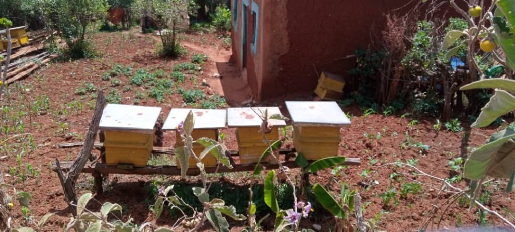
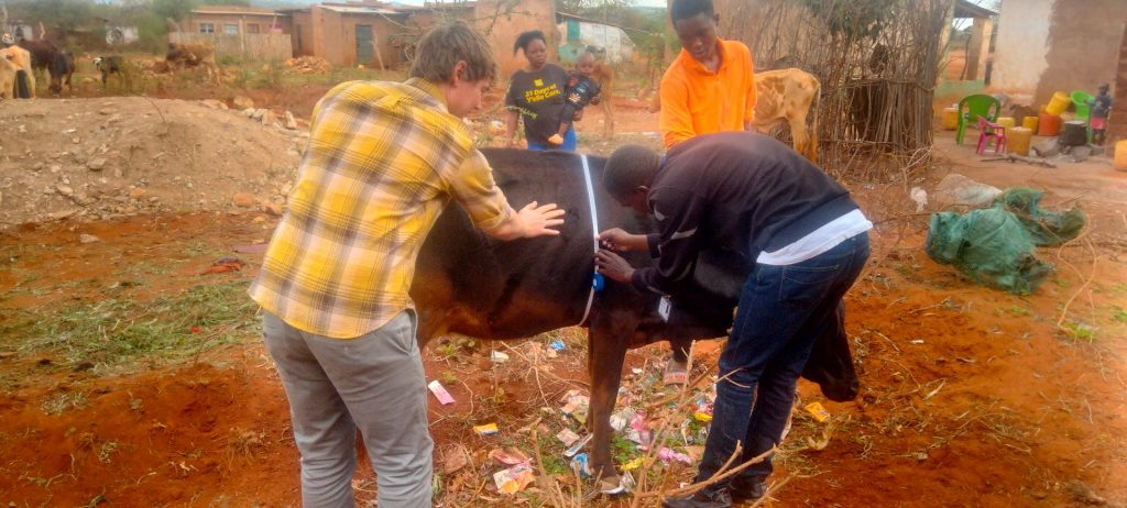
This blog describes an approach being developed to deliver rapid classification of farmer strategies. The data comes from a survey conducted with two groups of smallholder farmers (see image 2), one group living in the Taita Hills area of southern Kenya and the other in Yebelo, southern Ethiopia. This work would not have been possible without the support of my supervisors James Hammond, from the International Livestock Research Institute (ILRI) (and developer of the Rural Household Multi Indicator Survey, RHoMIS, used in this research), as well as Andrew Dowsey, Levi Wolf and Kate Robson Brown from the University of Bristol.
Image 2: Measuring a Cows Heart Girth as Part of the Farm Surveys
Aims of the project
The goal of my PhD is to contribute a landscape approach to analysing agricultural systems. On-farm practices are an important part of an agricultural system and are one of the trilogy of components that make-up what Rizzo et al (2022) call ‘agricultural landscape dynamics’ – the other two components being Natural Resources and Landscape Patterns. To understand how a farm interacts with and responds to Natural Resources and Landscape Patterns it seems sensible to try and understand not just each farms inputs and outputs but its overall strategy and component practices. (more…)
“Gaussian processes are a highly flexible class of non-parametric Bayesian models used in a variety of applications. In their exact form they provide principled uncertainty representations, at the expense of poor scalability (O(n^3)) with the number of training points. As a result, many approximate methods have been proposed to try and address this. We raise the question of how to assess the performance of such methods. The most obvious approach is to generate data from the exact GP model and then benchmark performance metrics of the approximations against the data generating process. Unfortunately, generating data from an exact GP is also in general an O(n^3) problem. We address this limitation by demonstrating how tunable parameters controlling the fidelity of inexact methods of drawing samples can be chosen to ensure that their samples are, with high probability, indistinguishable from genuine data from the exact GP.”
A post by Ben Griffiths, PhD student on the Compass programme.
My area of research is studying Quantile Generalised Additive Models (QGAMs), with my main application lying in energy demand forecasting. In particular, my focus is on developing faster and more stable fitting methods and model selection techniques. This blog post aims to briefly explain what QGAMs are, how to fit them, and a short illustrative example applying these techniques to data on extreme rainfall in Switzerland. I am supervised by Matteo Fasiolo and my research is sponsored by Électricité de France (EDF).
Quantile Generalised Additive Models
QGAMs are essentially the result of combining quantile regression (QR; performing regression on a specific quantile of the response) with a generalised additive model (GAM; fitting a model assuming additive smooth effects). Here we are in the regression setting, so let be the conditional c.d.f. of a response, , given a -dimensional vector of covariates, . In QR we model the th quantile, that is, .
Examples of true quantiles of SHASH distribution.
This might be useful in cases where we do not need to model the full distribution of and only need one particular quantile of interest (for example urban planners might only be interested in estimates of extreme rainfall e.g. ). It also allows us to make no assumptions about the underlying true distribution, instead we can model the distribution empirically using multiple quantiles.
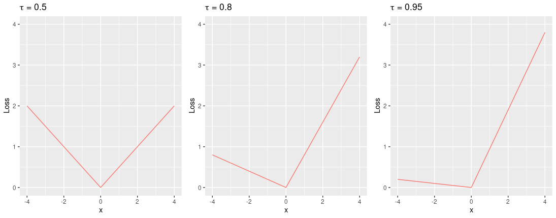
We can define the th quantile as the minimiser of expected loss
w.r.t. , where
is known as the pinball loss (Koenker, 2005).
Pinball loss for quantiles 0.5, 0.8, 0.95.
We can approximate the above expression empirically given a sample of size , which gives the quantile estimator, where
where is the th vector of covariates, and is vector of regression coefficients.
So far we have described QR, so to turn this into a QGAM we assume has additive structure, that is, we can write the th conditional quantile as
where the additive terms are defined in terms of basis functions (e.g. spline bases). A marginal smooth effect could be, for example
where are unknown coefficients, are known spline basis functions and is the basis dimension.
Denote the vector of basis functions evaluated at , then the design matrix is defined as having th row , for , and is the total basis dimension over all . Now the quantile estimate is defined as . When estimating the regression coefficients, we put a ridge penalty on to control complexity of , thus we seek to minimise the penalised pinball loss
where is a vector of positive smoothing parameters, is the learning rate and the ‘s are positive semi-definite matrices which penalise the wiggliness of the corresponding effect . Minimising with respect to given fixed and leads to the maximum a posteriori (MAP) estimator .
There are a number of methods to tune the smoothing parameters and learning rate. The framework from Fasiolo et al. (2021) consists in:
calibrating by Integrated Kullback–Leibler minimisation
selecting by Laplace Approximate Marginal Loss minimisation
estimating by minimising penalised Extended Log-F loss (note that this loss is simply a smoothed version of the pinball loss introduced above)
For more detail on what each of these steps means I refer the reader to Fasiolo et al. (2021). Clearly this three-layered nested optimisation can take a long time to converge, especially in cases where we have large datasets which is often the case for energy demand forecasting. So my project approach is to adapt this framework in order to make it less computationally expensive.
Application to Swiss Extreme Rainfall
Here I will briefly discuss one potential application of QGAMs, where we analyse a dataset consisting of observations of the most extreme 12 hourly total rainfall each year for 65 Swiss weather stations between 1981-2015. This data set can be found in the R package gamair and for model fitting I used the package mgcViz.
A basic QGAM for the 50% quantile (i.e. ) can be fitted using the following formula
where is the intercept term, is a parametric factor for climate region, are smooth effects, is the Annual North Atlantic Oscillation index, is the metres above sea level, is the year of observation, and and are the degrees east and north respectively.
After fitting in mgcViz, we can plot the smooth effects and see how these affect the extreme yearly rainfall in Switzerland.
Fitted smooth effects for North Atlantic Oscillation index, elevation, degrees east and north and year of observation.
From the plots observe the following; as we increase the NAO index we observe a somewhat oscillatory effect on extreme rainfall; when increasing elevation we see a steady increase in extreme rainfall before a sharp drop after an elevation of around 2500 metres; as years increase we see a relatively flat effect on extreme rainfall indicating the extreme rainfall patterns might not change much over time (hopefully the reader won’t regard this as evidence against climate change); and from the spatial plot we see that the south-east of Switzerland appears to be more prone to more heavy extreme rainfall.
We could also look into fitting a 3D spatio-temporal tensor product effect, using the following formula
where is the tensor product effect between , and . We can examine the spatial effect on extreme rainfall over time by plotting the smooths.
3D spatio-temporal tensor smooths for years 1985, 1995, 2005 and 2015.
There does not seem to be a significant interaction between the location and year, since we see little change between the plots, except for perhaps a slight decrease in the south-east.
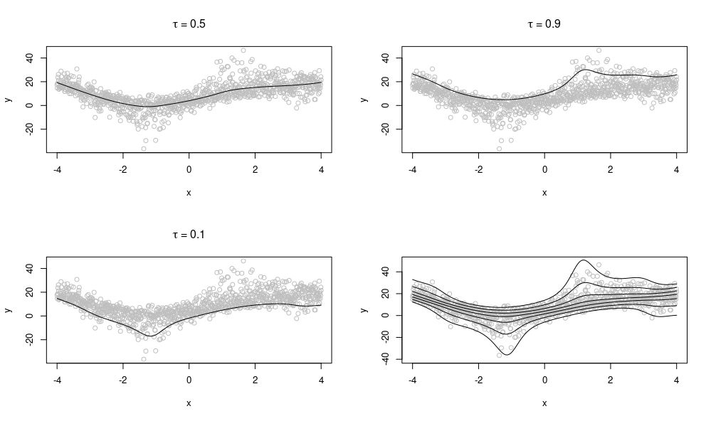
Finally, we can make the most of the QGAM framework by fitting multiple quantiles at once. Here we fit the first formula for quantiles , and we can examine the fitted smooths for each quantile on the spatial effect.
Spatial smooths for quantiles 0.1, 0.2, …, 0.9.
Interestingly the spatial effect is much stronger in higher quantiles than in the lower ones, where we see a relatively weak effect at the 0.1 quantile, and a very strong effect at the 0.9 quantile ranging between around -30 and +60.
The example discussed here is but one of many potential applications of QGAMs. As mentioned in the introduction, my research area is motivated by energy demand forecasting. My current/future research is focused on adapting the QGAM fitting framework to obtain faster fitting.
References
Fasiolo, M., S. N. Wood, M. Zaffran, R. Nedellec, and Y. Goude (2021). Fast calibrated additive quantile regression.Journal of the American Statistical Association 116(535), 1402–1412.
Koenker, R. (2005).Quantile Regression. Cambridge University Press.
Compass CDT is now recruiting for its fully funded places to start September 2023.
We are happy to announce that The University of Bristol online application system is open, and we are receiving applications for Compass CDT programme for September 2023 start. Early application is advised.
For 2023/34 entry, applicants must review the projects on offer. The projects are listed in the research section of our website. You will need to provide a Research Statement in your application documents with a ranked list of 3 projects of interest to you: 1 being the project of highest interest.
PhD Project Allocation Process
Application forms will be reviewed based on the 3 ranked projects specified. Successful applicants will be invited to attend an interview with the Compass admissions tutors and the specific project supervisor. If you are made an offer of PhD study it will be published through the online application system. You will then have 2 weeks to consider the offer before deciding whether to accept or decline.
The next review of applications for 2023 funded places will take place after
We welcome applications from all members of our community and are particularly encouraging those from diverse groups, such as members of the LGBT+ and black, Asian and minority ethnic communities, to join us.
Advantages of being a Compass Student
Stipend – a generous stipend of £21,668 pa tax free, paid in monthly payments. Plus your own expense budget of £1,000 pa towards travel and research activity.
No fees – all tuition fees are covered by the EPSRC and University of Bristol.
Bespoke training – first year units are designed specifically for the academic needs of each Compass student, which enables students to develop knowledge and capability to pursue cross-disciplinary PhD research.
Supervisors – supervisors from across academic disciplines offer a range of research projects.
Cohort – Compass students benefit from dedicated offices and collaboration spaces, enabling strong cohort links and opportunities for shared learning and research.
About Compass CDT
A 4-year bespoke PhD training programme in the statistical and computational techniques of data science, with partners from across the University of Bristol, industry and government agencies.
The cross-disciplinary programme offers exciting collaborations across medicine, computer science, geography, economics, life and earth sciences, as well as with our external partners who range from government organisations such as the Office for National Statistics, NCSC and the AWE, to industrial partners such as LV, Improbable, IBM Research, EDF, and AstraZeneca.
Students are co-located with the Institute for Statistical Science in the School of Mathematics, which occupies the Fry Building.
Hear from our students about their experience with the programme
Compass has allowed me to advance my statistical knowledge and apply it to a range of exciting applied projects, as well as develop skills that I’m confident will be highly useful for a future career in data science. – Shannon, Cohort 2
With the Compass CDT I feel part of a friendly, interactive environment that is preparing me for whatever I move on to next, whether it be in Academia or Industry. – Sam, Cohort 2
An incredible opportunity to learn the ever-expanding field of data science, statistics and machine learning amongst amazing people. – Danny, Cohort 1
APPLY BEFORE:
Wednesday 4 January 2023, 5pm (London, UK time zone)

=0")

")
")

")
![\mathbb{E}_V[\eta(w,V)]=g(w)](https://s0.wp.com/latex.php?latex=%5Cmathbb%7BE%7D_V%5B%5Ceta%28w%2CV%29%5D%3Dg%28w%29&bg=ffffff&fg=000000&s=0 "\mathbb{E}_V[\eta(w,V)]=g(w)")
![w_*=\underset{w}{\text{argmin}}\quad\mathbb{E}_V[\eta(w,V)].](https://s0.wp.com/latex.php?latex=w_%2A%3D%5Cunderset%7Bw%7D%7B%5Ctext%7Bargmin%7D%7D%5Cquad%5Cmathbb%7BE%7D_V%5B%5Ceta%28w%2CV%29%5D.&bg=ffffff&fg=000000&s=0 "w_*=\underset{w}{\text{argmin}}\quad\mathbb{E}_V[\eta(w,V)].")


") , is a data structure that consists of a set of nodes,
, is a data structure that consists of a set of nodes,  . Graphs are used to represent connections (edges) between objects (nodes), where the edges can be directed or undirected depending on whether the relationships between the nodes have direction. An
  node graph can be represented by an
  matrix, referred to as an adjacency matrix.
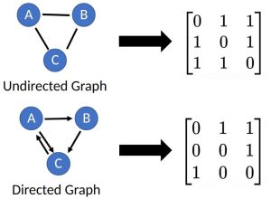
") be the conditional c.d.f. of a response,
be the conditional c.d.f. of a response,  , given a
  -dimensional vector of covariates,
  . In QR we model the
  th quantile, that is,
  = \inf \{y : F(y|\boldsymbol{x}) \geq \tau\}") .
.
 and only need one particular quantile of interest (for example urban planners might only be interested in estimates of extreme rainfall e.g.
  ). It also allows us to make no assumptions about the underlying true distribution, instead we can model the distribution empirically using multiple quantiles.
 = \mathbb{E} \left\{\rho_\tau (y - \mu)| \boldsymbol{x} \right \} = \int \rho_\tau(y - \mu) d F(y|\boldsymbol{x}),")
") , where
, where = (\tau - 1) z \boldsymbol{1}(z<0) + \tau z \boldsymbol{1}(z \geq 0),")
 = \boldsymbol{x}^\mathsf{T} \hat{\boldsymbol{\beta}}") where
where
 is the
  th vector of covariates, and
  is vector of regression coefficients.
") has additive structure, that is, we can write the
has additive structure, that is, we can write the  = \sum_{j=1}^m f_j(\boldsymbol{x}),")
 additive terms are defined in terms of basis functions (e.g. spline bases). A marginal smooth effect could be, for example
 = \sum_{k=1}^{r_j} \beta_{jk} b_{jk}(x_j),")
 are unknown coefficients,
 ") are known spline basis functions and
are known spline basis functions and  is the basis dimension.
 the vector of basis functions evaluated at
  design matrix
  is defined as having
  , and
, and  is the total basis dimension over all
  . Now the quantile estimate is defined as
  = \boldsymbol{\mathrm{x}}_i^\mathsf{T} \boldsymbol{\beta}") . When estimating the regression coefficients, we put a ridge penalty on
. When estimating the regression coefficients, we put a ridge penalty on  to control complexity of
  = \sum_{i=1}^n \frac{1}{\sigma} \rho_\tau \left\{y_i - \mu(\boldsymbol{x}_i)\right\} + \frac{1}{2} \sum_{j=1}^m \gamma_j \boldsymbol{\beta}^\mathsf{T} \boldsymbol{\mathrm{S}}_j \boldsymbol{\beta},")
") is a vector of positive smoothing parameters,
is a vector of positive smoothing parameters,  is the learning rate and the
  ‘s are positive semi-definite matrices which penalise the wiggliness of the corresponding effect
  and
and  leads to the maximum a posteriori (MAP) estimator
  .
. by Laplace Approximate Marginal Loss minimisation
 by minimising penalised Extended Log-F loss (note that this loss is simply a smoothed version of the pinball loss introduced above)
 ) can be fitted using the following formula
 + f_1(\mathrm{nao}_i) + f_2(\mathrm{el}_i) + f_3(\mathrm{Y}_i) + f_4(\mathrm{E}_i,\mathrm{N}_i),")
 is the intercept term,
 ") is a parametric factor for climate region,
is a parametric factor for climate region,  are smooth effects,
  is the Annual North Atlantic Oscillation index,
  is the metres above sea level,
  is the year of observation, and
  and
and  are the degrees east and north respectively.
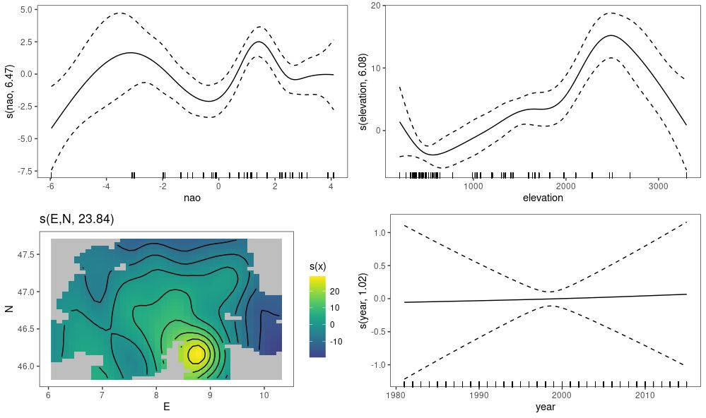
 + f_1(\mathrm{nao}_i) + f_2(\mathrm{el}_i) + t(\mathrm{E}_i,\mathrm{N}_i,\mathrm{Y}_i),")
 is the tensor product effect between
 , and we can examine the fitted smooths for each quantile on the spatial effect.