A post by Emma Ceccherini, PhD student on the Compass programme.
In December 2023, I attended NeurIPS, a machine learning conference, with some COMPASS colleagues. There, I attended a tutorial titled “Reconsidering Overfitting in the Age of Overparameterized Models”. The findings the speakers presented overturn some traditional statistical concepts, so I’d like to share some of these innovative ideas with the COMPASS blog readers.
Classical statistician vs deep learning practitioners
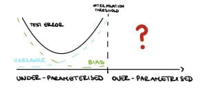
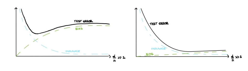
Classical statisticians argue that small models have high bias but large variance (Figure 1 (left)) and large models have low bias but high variance (Figure 1 (right)). This is called the bias-variance trade-off and is a crucial notion that can be found in all traditional statistic textbooks. Large, over-parameterised models perfectly interpolate the data points by fitting noise and they have a near-zero training error, but an increasing test error. This phenomenon is called overfitting and causes poor performances on unseen data. Overfitting implies low generalisation, which can be thought of as the model’s performance on newly generated data at test time.
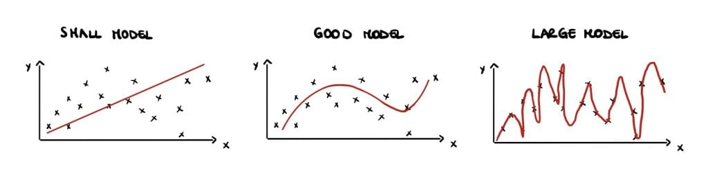
Therefore, statistics textbooks recommend avoiding overfitting and improving generalization by finding a balance in the bias-variance trade-off, either by reducing the number of parameters or using regularisation (Figure 1 (centre)).
However, as available computational power has increased, practitioners have made larger and larger models. For example, neural networks have millions of parameters, more than enough to fit noise, but they generalize very well in practice, performing significantly better than small models. These large over-parametrised models exceed the so-called interpolation threshold that is when the training error is approximately zero. Several theoretical statisticians are trying to infer what happens after this threshold. While we now have some answers, many questions are still up for debate!
The double descent
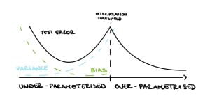
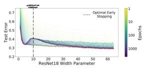
Nakkiran et al. [2019] show that in the under-parameterised regime, neural networks test errors exhibit the classical u-shape from the bias-variance trade-off, while in the over-parameterised regime, after the interpolation threshold, the test error decreases again creating the so-called double descent (see Figure 3). Figure 4 shows the test error of a neural network classifier on CIFAR-10, a standard image data set. The plot shows a double descent in the test error for neural networks trained until convergence (purple line).
The authors make two more innovative observations: harmless interpolation and good generalisation for large models. It can be observed from Figure 4 that regularisation, equivalent to early stopping (red line), is substantially beneficial around the interpolation threshold. However, as the model size grows the test error for optimal early stopped neural networks (red line) and the one of neural networks trained until convergence test (purple line) overlap. Therefore, For large models, interpolation (trained until convergence) is not worse than regularisation (optimal early stopped), that is interpolation is harmless. Finally, Figure 4 shows that the test error is low as the size of the model grows. Hence, for large models, we can achieve reasonably good test accuracy, namely as a result of good generalisation.
Given these groundbreaking experimental results, statisticians seek to use theoretical analysis to understand when these three phenomena occur. Although neural networks were the initial motivation of this work, they are hard to analyse even for shallow networks. And so statisticians resorted to understanding these phenomena starting from the well-known linear models.
Over-parameterisation in linear models of the form $\mathbf{Y} = \mathbf{X}\theta^* + \mathbf{W}$ means there are more features $d$ than number of samples $n$, i.e. $d >n$ for an input matrix $\mathbf{X}$ of dimension $n \times d$. Then the system $\mathbf{X}\hat{\theta} = \mathbf{Y}$ has infinite solutions, thus consider the solution with minimum norm $\hat{\theta} = \text{arg min}||\hat{\theta}||_2$.
After the interpolation threshold, the variance is dominating (see Figure 3) so it needs to go down for the test error to go down. Indeed, Bartlett et al. [2020] show that in this setup the variance decreases as $d \gg n$, precisely $$\text{variance} \asymp \frac{\sigma^2n}{d}. $$
It can be shown that data is approximately orthogonal when $d \gg n$, namely $<X_i, X_j> \approx 0$ for $i \neq 0$, so the noise “energy” is spread out along the $d$ dimensions, hence as $d$ grows the noise contribution decreases.
However, Bartlett et al. [2020] also show that the bias increases with $d$, precisely $$\text{bias} \asymp (1-\frac{n}{d})||\theta^*||_2^2.$$ This is because the signal “energy” as well is spread out along $d$ dimensions.
Eventually, the bias will dominate and the test error will increase again, see Figure 5 (left). Therefore under this framework, the double descent and harmless interpolation can be achieved but good generalisation cannot.
Finally, Bartlett et al. [2020] show that in the special case where the $k$ features are “upweighted”, all three phenomena are observed. Assuming a spiked covariance $$\Sigma = \mathbb{E}[\mathbf{X}\mathbf{X}^T] = \begin{bmatrix}
R\mathbf{I}_k & \mathbf{0} \\
\mathbf{0} & \mathbf{I}_{d-k}
\end{bmatrix},$$ it can be shown that the variance and the bias will go to zero as $d \rightarrow \infty$ provided that $R \gg \frac{d}{n}$, therefore the double descent, harmless interpolation and good generalization are achieved (see Figure 5 (right)).
Many unanswered questions remain
Similar results to the ones described for linear models have been obtained for linear classification [Muthukumar et al., 2021]. While these types of results for neural networks [Frei et al., 2022] are still limited. Moreover, there are still many open questions on benign overfitting for neural networks. For example, the existing result focuses on $d \gg n$ regimes for neural networks, but there are no results on neural networks over-parameterised in low dimensions by increasing their width. Theoretical statisticians still have plenty of work to do to fully understand these phenomena!
References
Peter L. Bartlett, Philip M. Long, G´abor Lugosi, and Alexander Tsigler. Benign overfitting in linear
regression. Proceedings of the National Academy of Sciences, 117(48):30063–30070, April 2020. ISSN
1091-6490. doi: 10.1073/pnas.1907378117. URL http://dx.doi.org/10.1073/pnas.1907378117.
Spencer Frei, Gal Vardi, Peter L. Bartlett, Nathan Srebro, and Wei Hu. Implicit bias in leaky relu
networks trained on high-dimensional data, 2022.
Vidya Muthukumar, Adhyyan Narang, Vignesh Subramanian, Mikhail Belkin, Daniel Hsu, and Anant
Sahai. Classification vs regression in overparameterized regimes: Does the loss function matter?,
2021.
Preetum Nakkiran, Gal Kaplun, Yamini Bansal, Tristan Yang, Boaz Barak, and Ilya Sutskever. Deep
double descent: Where bigger models and more data hurt, 2019.
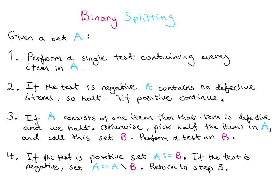
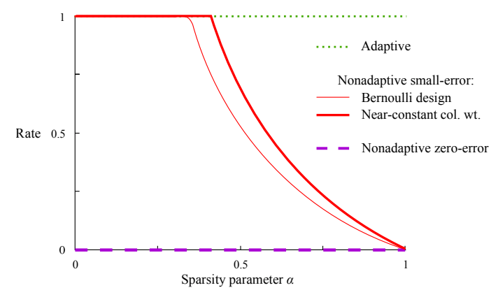 A graph comparing different group testing designs, where the $\text{Rate} = \log_2\binom{n}{k}/T$ where $T$ is the number of tests needed to recover all the defective items (with high probability for the red lines and with certainty for the purple line). [1]


 with a particular sequence, we can take a sample from this synthesis and analyse it via mass spectrometry. In this process, molecules in the sample are first fragmented — broken apart into ions — and these charged fragments are then passed through an electromagnetic field. The trajectory of each fragment through this field depends on its mass/charge ratio (m/z), so measuring these trajectories (e.g. by measuring time of flight before hitting some detector) allows us to calculate the m/z of fragments in the sample. This gives us a discrete mass spectrum: counts of detected fragments (intensity) across a range of m/z bins [5].
 every product of a single fragmentation of
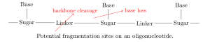
 , where
  is the intensity in the
  bin. For a set
  of possible fragments, let
  be the amount of
  that is actually present. We would like to estimate the amounts of each fragment based on the spectrum
  .
. and
and  and this produced a spectrum
  , we can say the intensity contributed to bin
  by
by  In mass spectrometry, the intensity in a single bin due to a single fragment is linear in the amount of that fragment, and the intensities in a single bin due to different fragments are additive, so in some general spectrum we have
 such that
  (so the columns of
  correspond to fragments in
  solves
  . In practice this exact solution is not found — due to experimental noise and potentially because there are contaminant fragments in the sample not included in
  for which
  is close to
  -normalise these columns, meaning the total intensity (over all bins) of each fragment in the library matrix is uniform, and so the values in
  can be directly interpreted as relative abundances of each fragment.
 which maximises the likelihood of the system is approximated by the iterative formula
}=\left(\mathbf A^T \frac{\mathbf b}{\mathbf{A\hat x}^{(t)}}\right)\odot \mathbf{\hat x}^{(t)}.")
 represent (respectively) elementwise division and multiplication of two vectors. This is known as the Richardson-Lucy algorithm [9].
}=\left(\mathbf A^T \frac{\mathbf b}{\mathbf{A\hat x}^{(t)}}\right)\odot \frac{ \mathbf{\hat x}^{(t)}}{\mathbf 1 + \lambda},")
 is a regularisation parameter [10].
 , we smooth and bin the m/z values of the most abundant isotopes of
  , and store these values in the columns of
  ) for clarity.
 on some space
  with probability density functions (PDFs)
  respectively, the density ratio is the function
  defined by
:=\frac{p_0(z)}{p_1(z)}") .
.
 and
and  to estimate
  . What makes DRE so useful is that it gives us a way to characterise the difference between these 2 classes of data using just 1 quantity,
 ") and
and  by
by  . The task of predicting
  given
given  is then our standard classification problem. In classification a common target is the Bayes Optimal Classifier, the classifier
  which maximises
 ).") We can write this classifier in terms of
We can write this classifier in terms of =\mathbb{I}\{\mathbb{P}(Y=1|Z=z)>0.5\}") where
where  is the indicator function. Then, by the total law of probability, we have
=\frac{p_{Z|Y=1}(z)\mathbb{P}(Y=1)}{p_{Z|Y=1}(z)\mathbb{P}(Y=1)+p_{Z|Y=0}(z)\mathbb{P}(Y=0)}")
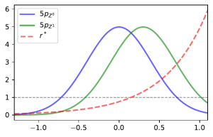
\mathbb{P}(Y=1)}{p_1(z)\mathbb{P}(Y=1)+p_0(z)\mathbb{P}(Y=0)} =\frac{1}{1+\frac{1}{r}\frac{\mathbb{P}(Y=0)}{\mathbb{P}(Y=1)}}.")
 , if
, if  is “close” to
  then
then  is a good estimate of
 ")
p_0(z)\mathrm{d}z=1")
") represent the KL divergence from
represent the KL divergence from  to
to  . The constraint ensures that the right hand side of our KL divergence is indeed a PDF. From the definition of the KL-divergence we can rewrite the solution to this as
 ![\hat r:=\frac{\tilde r}{\mathbb{E}[r(X^0)]}](https://s0.wp.com/latex.php?latex=%5Chat+r%3A%3D%5Cfrac%7B%5Ctilde+r%7D%7B%5Cmathbb%7BE%7D%5Br%28X%5E0%29%5D%7D&bg=ffffff&fg=000000&s=0 "\hat r:=\frac{\tilde r}{\mathbb{E}[r(X^0)]}") where
where  is the solution to the unconstrained optimisation
![\underset{r}{\text{min}}~\mathbb{E}[\log (r(Z^1))]-\log(\mathbb{E}[r(Z^0)]).](https://s0.wp.com/latex.php?latex=%5Cunderset%7Br%7D%7B%5Ctext%7Bmin%7D%7D%7E%5Cmathbb%7BE%7D%5B%5Clog+%28r%28Z%5E1%29%29%5D-%5Clog%28%5Cmathbb%7BE%7D%5Br%28Z%5E0%29%5D%29.&bg=ffffff&fg=000000&s=2 "\underset{r}{\text{min}}~\mathbb{E}[\log (r(Z^1))]-\log(\mathbb{E}[r(Z^0)]).")
 from
from  and samples
  from
from  our estimate of the density ratio will be
 \right)^{-1}\tilde r") where
where )-\log\left(\frac{1}{n}\sum_{i=1}^n r(z^0_i)\right).")
 . We assume that
 =1") so that either
so that either =\varphi(z)") with
with ") not constant and refer to
not constant and refer to  as the missingness function. This type of missingness is known as missing not at random (MNAR) and when dealt with improperly can lead to biased result. Some examples of MNAR data could be readings take from a medical instrument which is more likely to err when attempting to read extreme values or recording responses to a questionnaire where respondents may be more likely to not answer if the deem their response to be unfavourable. Note that while we do not see what the true response would be, we do at least get a response meaning that we know when an observation is missing.
 we observe samples from their corrupted versions
  . We take their respective missingness functions to be
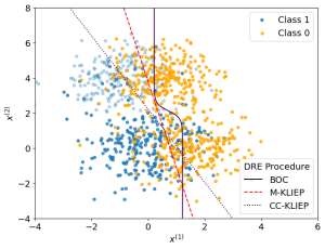
  and assume them to be known. Now let us look at what would happen if we implemented KLIEP with the data naively by simply filtering out the missing-values. In this case, the actual density ratio we would be estimating would be
:=\frac{p_{X_1|X_1\neq\varnothing}(z)}{p_{X_0|X_o\neq\varnothing}(z)}\propto\frac{(1-\varphi_1(z))p_1(z)}{(1-\varphi_0(z))p_0(z)}\not{\propto}r^*(z)")
 are more likely to be missing when larger and class
  has no missingness.
![\mathbb{E}[g(Z)]=\mathbb{E}\left[\frac{\mathbb{I}\{X\neq\varnothing\}g(X)}{1-\varphi(X)}\right].](https://s0.wp.com/latex.php?latex=%5Cmathbb%7BE%7D%5Bg%28Z%29%5D%3D%5Cmathbb%7BE%7D%5Cleft%5B%5Cfrac%7B%5Cmathbb%7BI%7D%5C%7BX%5Cneq%5Cvarnothing%5C%7Dg%28X%29%7D%7B1-%5Cvarphi%28X%29%7D%5Cright%5D.&bg=ffffff&fg=000000&s=2 "\mathbb{E}[g(Z)]=\mathbb{E}\left[\frac{\mathbb{I}\{X\neq\varnothing\}g(X)}{1-\varphi(X)}\right].")
 from
from  and samples
  from
from  our estimate is
 }{1-\varphi_o(x_i^o)}\right)^{-1}\tilde r") where
where )}{1-\varphi_1(x_i^1)}-\log\left(\frac{1}{n}\sum_{i=1}^n\frac{\mathbb{I}\{x_i^0\neq\varnothing\}r(x_i^0)}{1-\varphi_0(x_i^0)}\right).")
 .
. . That is, the dimension of the embeddings (
 ) is much smaller than the number of items or users. The hope is that the position of these embeddings captures some of the latent (hidden) structure of the items/users, and so similar items end up ‘close together’ in the embedding space. What is meant by being ‘close’ may be specified by some similarity measure.
 users
users ") and a group of
and a group of  items
items ") . Then we let
. Then we let  be the ratings matrix where position
  represents whether user
  interacts with item
  is very sparse, since most users only interact with a small subset of the full item set
  . For any items
  , and item embeddings,
  , is Matrix Factorisation. The idea is to find low-rank embeddings such that the product
  is a good approximation to the ratings matrix
  = \sum_{u, i} \left(R_{ui} - \langle X_u, Y_i \rangle \right)^2.")
 .
. and
and  , we can look at the row of
  , i.e.
,")
 and
and  ,
,}{1 + \exp(\langle X_u, Y_i \rangle + \beta_u + \beta_i)} \right).")
=0") given “noisy” measurements of
given “noisy” measurements of  [2].
[2].") , knows that it is differentiable and admits an unique minimum – hence the problem
, knows that it is differentiable and admits an unique minimum – hence the problem")
 , consider an unbiased estimator
 ") s.t.
s.t. ![\mathbb{E}_V[\eta(w,V)]=g(w)](https://s0.wp.com/latex.php?latex=%5Cmathbb%7BE%7D_V%5B%5Ceta%28w%2CV%29%5D%3Dg%28w%29&bg=ffffff&fg=000000&s=0 "\mathbb{E}_V[\eta(w,V)]=g(w)") and to rewrite the problem as
and to rewrite the problem as![w_*=\underset{w}{\text{argmin}}\quad\mathbb{E}_V[\eta(w,V)].](https://s0.wp.com/latex.php?latex=w_%2A%3D%5Cunderset%7Bw%7D%7B%5Ctext%7Bargmin%7D%7D%5Cquad%5Cmathbb%7BE%7D_V%5B%5Ceta%28w%2CV%29%5D.&bg=ffffff&fg=000000&s=0 "w_*=\underset{w}{\text{argmin}}\quad\mathbb{E}_V[\eta(w,V)].")
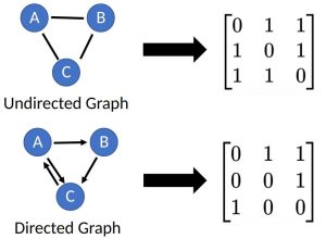
") , is a data structure that consists of a set of nodes,
, is a data structure that consists of a set of nodes,  . Graphs are used to represent connections (edges) between objects (nodes), where the edges can be directed or undirected depending on whether the relationships between the nodes have direction. An
  matrix, referred to as an adjacency matrix.