Student Perspectives: Density Ratio Estimation with Missing Data

Posted on 3rd July 20233rd July 2023 by josh.givens

A post by Josh Givens, PhD student on the Compass programme.

Density ratio estimation is a highly useful field of mathematics with many applications. This post describes my research undertaken alongside my supervisors Song Liu and Henry Reeve which aims to make density ratio estimation robust to missing data. This work was recently published in proceedings for AISTATS 2023.

Density Ratio Estimation

Definition

As the name suggests, density ratio estimation is simply the task of estimating the ratio between two probability densities. More precisely for two RVs (Random Variables) $Z^0, Z^1$ on some space $\mathcal{Z}$ with probability density functions (PDFs) $p_0, p_1$ respectively, the density ratio is the function $r^*:\mathcal{Z}\rightarrow\mathbb{R}$ defined by

$r^*(z):=\frac{p_0(z)}{p_1(z)}$ .

Plot of the scaled density ratio alongside the PDFs for the two classes.

Density ratio estimation (DRE) is then the practice of using IID (independent and identically distributed) samples from $Z^0$ and $Z^1$ to estimate $r^*$ . What makes DRE so useful is that it gives us a way to characterise the difference between these 2 classes of data using just 1 quantity, $r^*$ .

The Density Ratio in Classification

We now give demonstrate this characterisability in the case of classification. To frame this as a classification problem define $Y\sim\text{Bernoulli}(0.5)$ and $Z$ by $Z|Y=y\sim Z^{y}$ . The task of predicting $Y$ given $Z$ using some function $\phi:\mathcal{Z}\rightarrow\{0,1\}$ is then our standard classification problem. In classification a common target is the Bayes Optimal Classifier, the classifier $\phi^*$ which maximises $\mathbb{P}(Y=\phi(Z)).$ We can write this classifier in terms of $r^*$ as we know that $\phi^*(z)=\mathbb{I}\{\mathbb{P}(Y=1|Z=z)>0.5\}$ where $\mathbb{I}$ is the indicator function. Then, by the total law of probability, we have

$\mathbb{P}(Y=1|Z=z)=\frac{p_{Z|Y=1}(z)\mathbb{P}(Y=1)}{p_{Z|Y=1}(z)\mathbb{P}(Y=1)+p_{Z|Y=0}(z)\mathbb{P}(Y=0)}$

$=\frac{p_1(z)\mathbb{P}(Y=1)}{p_1(z)\mathbb{P}(Y=1)+p_0(z)\mathbb{P}(Y=0)} =\frac{1}{1+\frac{1}{r}\frac{\mathbb{P}(Y=0)}{\mathbb{P}(Y=1)}}.$

Hence to learn the Bayes optimal classifier it is sufficient to learn the density ratio and a constant. This pattern extends well beyond Bayes optimal classification to many other areas such as error controlled classification, GANs, importance sampling, covariate shift, and others. Generally speaking, if you are in any situation where you need to characterise the difference between two classes of data, it’s likely that the density ratio will make an appearance.

Estimation Implementation – KLIEP

Now we have properly introduced and motivated DRE, we need to look at how we can go about performing it. We will focus on one popular method called KLIEP here but there are a many different methods out there (see Sugiyama et al 2012 for some additional examples.)

The intuition behind KLIEP is simple: as $r^* \cdot p_0=p_1$ , if $\hat r\cdot p_0$ is “close” to $p_1$ then $\hat r$ is a good estimate of $r^*$ . To measure this notion of closeness KLIEP uses the KL (Kullback-Liebler) divergence which measures the distance between 2 probability distributions. We can now formulate our ideal KLIEP objective as follows:

$\underset{r}{\text{min}}~ KL(p_1|p_0\cdot r)$

$\text{subject to:}~ \int_{\mathcal{Z}}r(z)p_0(z)\mathrm{d}z=1$

where $KL(p|p')$ represent the KL divergence from $p$ to $p'$ . The constraint ensures that the right hand side of our KL divergence is indeed a PDF. From the definition of the KL-divergence we can rewrite the solution to this as $\hat r:=\frac{\tilde r}{\mathbb{E}[r(X^0)]}$ where $\tilde r$ is the solution to the unconstrained optimisation

$\underset{r}{\text{min}}~\mathbb{E}[\log (r(Z^1))]-\log(\mathbb{E}[r(Z^0)]).$

As this is now just an unconstrained optimisation over expectations of known transformations of $Z^0, Z^1$ , we can approximate this using samples. Given samples $z^0_1,\dotsc,z^0_n$ from $Z_0$ and samples $z^1_1,\dotsc,z^1_n$ from $Z_1$ our estimate of the density ratio will be $\hat r:=\left(\frac{1}{n}\sum_{i=1}^nr(z_i^0)\right)^{-1}\tilde r$ where $\tilde r$ solves

$\underset{r}{\min}~ \frac{1}{n}\sum_{i=1}^n \log(r(z^1_i))-\log\left(\frac{1}{n}\sum_{i=1}^n r(z^0_i)\right).$

Despite KLIEP being commonly used, up until now it has not been made robust to missing not at random data. This is what our research aims to do.

Missing Data

Suppose that instead of observing samples from $Z$ , we observe samples from some corrupted version of $Z$ , $X$ . We assume that $\mathbb{P}(\{X=\varnothing\}\cup \{X=Z\})=1$ so that either $X$ is missing or $X$ takes the value of $Z$ . We also assume that whether $X$ is missing depends upon the value of $Z$ . Specifically we assume $\mathbb{P}(X=\varnothing|Z=z)=\varphi(z)$ with $\varphi(z)$ not constant and refer to $\varphi$ as the missingness function. This type of missingness is known as missing not at random (MNAR) and when dealt with improperly can lead to biased result. Some examples of MNAR data could be readings take from a medical instrument which is more likely to err when attempting to read extreme values or recording responses to a questionnaire where respondents may be more likely to not answer if the deem their response to be unfavourable. Note that while we do not see what the true response would be, we do at least get a response meaning that we know when an observation is missing.

Missing Data with DRE

We now go back to density ratio estimation in the case where instead of observing samples from $Z^0,Z^1$ we observe samples from their corrupted versions $X^0, X^1$ . We take their respective missingness functions to be $\varphi_0, \varphi_1$ and assume them to be known. Now let us look at what would happen if we implemented KLIEP with the data naively by simply filtering out the missing-values. In this case, the actual density ratio we would be estimating would be

$r'(z):=\frac{p_{X_1|X_1\neq\varnothing}(z)}{p_{X_0|X_o\neq\varnothing}(z)}\propto\frac{(1-\varphi_1(z))p_1(z)}{(1-\varphi_0(z))p_0(z)}\not{\propto}r^*(z)$

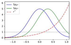
and so we would get inaccurate estimates of the density ratio no matter how many samples are used to estimate it. The image below demonstrates this in the case were samples in class $1$ are more likely to be missing when larger and class $0$ has no missingness.

A plot of the density ratio using both the full data and only the observed part of the corrupted data

Our Solution

Our solution to this problem is to use importance weighting. Using relationships between the densities of $X$ and $Z$ we have that

$\mathbb{E}[g(Z)]=\mathbb{E}\left[\frac{\mathbb{I}\{X\neq\varnothing\}g(X)}{1-\varphi(X)}\right].$

As such we can re-write the KLIEP objective to keep our expectation estimation unbiased even when using these corrupted samples. This gives our modified objective which we call M-KLIEP as follows. Given samples $x^0_1,\dotsc,x^0_n$ from $X_0$ and samples $x^1_1,\dotsc,x^1_n$ from $X_1$ our estimate is $\hat r=\left(\frac{1}{n}\sum_{i=1}^n\frac{\mathbb{I}\{x_i^0\neq\varnothing\}r(x_i^0)}{1-\varphi_o(x_i^o)}\right)^{-1}\tilde r$ where $\tilde r$ solves

$\underset{r}{\min}~\frac{1}{n}\sum_{i=1}^n\frac{\mathbb{I}\{x_i^1\neq\varnothing\}\log(r(x_i^1))}{1-\varphi_1(x_i^1)}-\log\left(\frac{1}{n}\sum_{i=1}^n\frac{\mathbb{I}\{x_i^0\neq\varnothing\}r(x_i^0)}{1-\varphi_0(x_i^0)}\right).$

This objective will now target $r^*$ even when used on MNAR data.

Application to Classification

We now apply our density ratio estimation on MNAR data to estimate the Bayes optimal classifier. Below shows a plot of samples alongside the true Bayes optimal classifier and estimated classifiers from the samples via our method M-KLIEP and a naive method CC-KLIEP which simply ignores missing points. Missing data points are faded out.

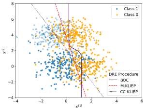
Faded points represent missing values. M-KLIEP represents our method, CC-KLIEP represents a Naive approach, BOC gives the Bayes optimal classifier

As we can see, due to not accounting for the MNAR nature of the data, CC-KLIEP underestimates the true number of class 1 samples in the top left region and therefore produces a worse classifier than our approach.

Additional Contributions

As well as this modified objective our paper provides the following additional contributions:

Theoretical finite sample bounds on the accuracy of our modified procedure.
Methods for learning the missingness functions $\varphi_1,\varphi_0$ .
Expansions to partial missingness via a Naive-Bayes framework.
Downstream implementation of our method within Neyman-Pearson classification.
Adaptations to Neyman-Pearson classification itself making it robust to MNAR data.

For more details see our paper and corresponding github repository. If you have any questions on this work feel free to contact me at josh.givens@bristol.ac.uk.

References

Givens, J., Liu, S., & Reeve, H. W. J. (2023). Density ratio estimation and neyman pearson classification with missing data. In F. Ruiz, J. Dy, & J.-W. van de Meent (Eds.), Proceedings of the 26th international conference on artificial intelligence and statistics (Vol. 206, pp. 8645–8681). PMLR.

Sugiyama, M., Suzuki, T., & Kanamori, T. (2012). Density Ratio Estimation in Machine Learning. Cambridge University Press.

Student Perspectives: Intro to Recommendation Systems

Posted on 12th May 202312th May 2023 by hannah.sansford

A post by Hannah Sansford, PhD student on the Compass programme.

Introduction

Like many others, I interact with recommendation systems on a daily basis; from which toaster to buy on Amazon, to which hotel to book on booking.com, to which song to add to a playlist on Spotify. They are everywhere. But what is really going on behind the scenes?

Recommendation systems broadly fit into two main categories:

1) Content-based filtering. This approach uses the similarity between items to recommend items similar to what the user already likes. For instance, if Ed watches two hair tutorial videos, the system can recommend more hair tutorials to Ed.

2) Collaborative filtering. This approach uses the the similarity between users’ past behaviour to provide recommendations. So, if Ed has watched similar videos to Ben in the past, and Ben likes a cute cat video, then the system can recommend the cute cat video to Ed (even if Ed hasn’t seen any cute cat videos).

Both systems aim to map each item and each user to an embedding vector in a common low-dimensional embedding space $E = \mathbb{R}^d$ . That is, the dimension of the embeddings ( $d$ ) is much smaller than the number of items or users. The hope is that the position of these embeddings captures some of the latent (hidden) structure of the items/users, and so similar items end up ‘close together’ in the embedding space. What is meant by being ‘close’ may be specified by some similarity measure.

Collaborative filtering

In this blog post we will focus on the collaborative filtering system. We can break it down further depending on the type of data we have:

1) Explicit feedback data: aims to model relationships using explicit data such as user-item (numerical) ratings.

2) Implicit feedback data: analyses relationships using implicit signals such as clicks, page views, purchases, or music streaming play counts. This approach makes the assumption that: if a user listens to a song, for example, they must like it.

The majority of the data on the web comes from implicit feedback data, hence there is a strong demand for recommendation systems that take this form of data as input. Furthermore, this form of data can be collected at a much larger scale and without the need for users to provide any extra input. The rest of this blog post will assume we are working with implicit feedback data.

Problem Setup

Suppose we have a group of $n$ users $U = (u_1, \ldots, u_n)$ and a group of $m$ items $I = (i_1, \ldots, i_m)$ . Then we let $\mathbf{R} \in \mathbb{R}^{n \times m}$ be the ratings matrix where position $R_{ui}$ represents whether user $u$ interacts with item $i$ . Note that, in most cases the matrix $\mathbf{R}$ is very sparse, since most users only interact with a small subset of the full item set $I$ . For any items $i$ that user $u$ does not interact with, we set $R_{ui}$ equal to zero. To be clear, a value of zero does not imply the user does not like the item, but that they have not interacted with it. The final goal of the recommendation system is to find the best recommendations for each user of items they have not yet interacted with.

Matrix Factorisation (MF)

A simple model for finding user emdeddings, $\mathbf{X} \in \mathbb{R}^{n \times d}$ , and item embeddings, $\mathbf{Y} \in \mathbb{R}^{m \times d}$ , is Matrix Factorisation. The idea is to find low-rank embeddings such that the product $\mathbf{XY}^\top$ is a good approximation to the ratings matrix $\mathbf{R}$ by minimising some loss function on the known ratings.

A natural loss function to use would be the squared loss, i.e.

$L(\mathbf{X}, \mathbf{Y}) = \sum_{u, i} \left(R_{ui} - \langle X_u, Y_i \rangle \right)^2.$

This corresponds to minimising the Frobenius distance between $\mathbf{R}$ and its approximation $\mathbf{XY}^\top$ , and can be solved easily using the singular value decomposition $\mathbf{R} = \mathbf{U S V}^\top$ .

Once we have our embeddings $\mathbf{X}$ and $\mathbf{Y}$ , we can look at the row of $\mathbf{XY}^\top$ corresponding to user $u$ and recommend the items corresponding to the highest values (that they haven’t already interacted with).

Logistic MF

Minimising the loss function in the previous section is equivalent to modelling the probability that user $u$ interacts with item $i$ as the inner product $\langle X_u, Y_i \rangle$ , i.e.

$R_{ui} \sim \text{Bernoulli}(\langle X_u, Y_i \rangle),$

and maximising the likelihood over $\mathbf{X}$ and $\mathbf{Y}$ .

In a research paper from Spotify [3], this relationship is instead modelled according to a logistic function parameterised by the sum of the inner product above and user and item bias terms, $\beta_u$ and $\beta_i$ ,

$R_{ui} \sim \text{Bernoulli} \left( \frac{\exp(\langle X_u, Y_i \rangle + \beta_u + \beta_i)}{1 + \exp(\langle X_u, Y_i \rangle + \beta_u + \beta_i)} \right).$

Relation to my research

A recent influential paper [1] proved an impossibility result for modelling certain properties of networks using a low-dimensional inner product model. In my 2023 AISTATS publication [2] we show that using a kernel, such as the logistic one in the previous section, to model probabilities we can capture these properties with embeddings lying on a low-dimensional manifold embedded in infinite-dimensional space. This has various implications, and could explain part of the success of Spotify’s logistic kernel in producing good recommendations.

References

[1] Seshadhri, C., Sharma, A., Stolman, A., and Goel, A. (2020). The impossibility of low-rank representations for triangle-rich complex networks. Proceedings of the National Academy of Sciences, 117(11):5631–5637.

[2] Sansford, H., Modell, A., Whiteley, N., and Rubin-Delanchy, P. (2023). Implications of sparsity and high triangle density for graph representation learning. Proceedings of The 26th International Conference on Artificial Intelligence and Statistics, PMLR 206:5449-5473.

[3] Johnson, C. C. (2014). Logistic matrix factorization for implicit feedback data. Advances in Neural Information Processing Systems, 27(78):1–9.

Student Perspectives: An Introduction to Stochastic Gradient Methods

Posted on 14th March 202315th March 2023 by ettore.fincato

A post by Ettore Fincato, PhD student on the Compass programme.

This post provides an introduction to Gradient Methods in Stochastic Optimisation. This class of algorithms is the foundation of my current research work with Prof. Christophe Andrieu and Dr. Mathieu Gerber, and finds applications in a great variety of topics, such as regression estimation, support vector machines, convolutional neural networks.

We can see below a simulation by Emilien Dupont (https://emiliendupont.github.io/) which represents two trajectories of an optimisation process of a time-varying function. This well describes the main idea behind the algorithms we will be looking at, that is, using the (stochastic) gradient of a (random) function to iteratively reach the optimum.

Stochastic Optimisation

Stochastic optimisation was introduced by [1], and its aim is to find a scheme for solving equations of the form $\nabla_w g(w)=0$ given “noisy” measurements of $g$ [2].

In the simplest deterministic framework, one can fully determine the analytical form of $g(w)$ , knows that it is differentiable and admits an unique minimum – hence the problem

$w_*=\underset{w}{\text{argmin}}\quad g(w)$

is well defined and solved by $\nabla_w g(w)=0$ .

On the other hand, one may not be able to fully determine $g(w)$ because his experiment is corrupted by a random noise. In such cases, it is common to identify this noise with a random variable, say $V$ , consider an unbiased estimator $\eta(w,V)$ s.t. $\mathbb{E}_V[\eta(w,V)]=g(w)$ and to rewrite the problem as

$w_*=\underset{w}{\text{argmin}}\quad\mathbb{E}_V[\eta(w,V)].$

(more…)

Student Perspectives: An Introduction to Graph Neural Networks (GNNs)

Posted on 17th February 202317th February 2023 by emerald.dilworth

A post by Emerald Dilworth, PhD student on the Compass programme.

This blog post serves as an accessible introduction to Graph Neural Networks (GNNs). An overview of what graph structured data looks like, distributed vector representations, and a quick description of Neural Networks (NNs) are given before GNNs are introduced.

An Introductory Overview of GNNs:

You can think of a GNN as a Neural Network that runs over graph structured data, where we know features about the nodes – e.g. in a social network, where people are nodes, and edges are them sharing a friendship, we know things about the nodes (people), for instance their age, gender, location. Where a NN would just take in the features about the nodes as input, a GNN takes in this in addition to some known graph structure the data has. Some examples of GNN uses include:

Predictions of a binary task – e.g. will this molecule (which the structure of can be represented by with a graph) inhibit this given bacteria? The GNN can then be used to predict for a molecule not trained on. Finding a new antibiotic is one of the most famous papers using GNNs [1].
Social networks and recommendation systems, where GNNs are used to predict new links [2].

What is a Graph?

A graph, $G = (V,E)$ , is a data structure that consists of a set of nodes, $V$ , and a set of edges, $E$ . Graphs are used to represent connections (edges) between objects (nodes), where the edges can be directed or undirected depending on whether the relationships between the nodes have direction. An $n$ node graph can be represented by an $n \times n$ matrix, referred to as an adjacency matrix.

Idea of Distributed Vector Representations

In machine learning architectures, the data input often needs to be converted to a tensor for the model, e.g. via 1-hot encoding. This provides an input (or local) representation of the data, which if we think about 1-hot encoding creates a large, sparse representation of 0s and 1s. The input representation is a discrete representation of objects, but lacks information on how things are correlated, how related they are, what they have in common. Often, machine learning models learn a distributed representation, where it learns how related objects are; nodes that are similar will have similar distributed representations. (more…)

Student Perspectives: An Introduction to Deep Kernel Machines

Posted on 17th January 202317th January 2023 by edward.milsom

A post by Edward Milsom, PhD student on the Compass programme.

This blog post provides a simple introduction to Deep Kernel Machines[1] (DKMs), a novel supervised learning method that combines the advantages of both deep learning and kernel methods. This work provides the foundation of my current research on convolutional DKMs, which is supervised by Dr Laurence Aitchison.

Why aren’t kernels cool anymore?

Kernel methods were once top-dog in machine learning due to their ability to implicitly map data to complicated feature spaces, where the problem usually becomes simpler, without ever explicitly computing the transformation. However, in the past decade deep learning has become the new king for complicated tasks like computer vision and natural language processing.

Neural networks are flexible when learning representations

The reason is twofold: First, neural networks have millions of tunable parameters that allow them to learn their feature mappings automatically from the data, which is crucial for domains like images which are too complex for us to specify good, useful features by hand. Second, their layer-wise structure means these mappings can be built up to increasingly more abstract representations, while each layer itself is relatively simple[2]. For example, trying to learn a single function that takes in pixels from pictures of animals and outputs their species is difficult; it is easier to map pixels to corners and edges, then shapes, then body parts, and so on.

Kernel methods are rigid when learning representations

It is therefore notable that classical kernel methods lack these characteristics: most kernels have a very small number of tunable hyperparameters, meaning their mappings cannot flexibly adapt to the task at hand, leaving us stuck with a feature space that, while complex, might be ill-suited to our problem. (more…)

Student Perspectives: Spectral Clustering for Rapid Identification of Farm Strategies

Posted on 19th December 202212th January 2023 by dan.milner

A post by Dan Milner, PhD student on the Compass programme.

Image 1: Smallholder Farm – Yebelo, southern Ethiopia

Introduction

This blog describes an approach being developed to deliver rapid classification of farmer strategies. The data comes from a survey conducted with two groups of smallholder farmers (see image 2), one group living in the Taita Hills area of southern Kenya and the other in Yebelo, southern Ethiopia. This work would not have been possible without the support of my supervisors James Hammond, from the International Livestock Research Institute (ILRI) (and developer of the Rural Household Multi Indicator Survey, RHoMIS, used in this research), as well as Andrew Dowsey, Levi Wolf and Kate Robson Brown from the University of Bristol.

Image 2: Measuring a Cows Heart Girth as Part of the Farm Surveys

Aims of the project

The goal of my PhD is to contribute a landscape approach to analysing agricultural systems. On-farm practices are an important part of an agricultural system and are one of the trilogy of components that make-up what Rizzo et al (2022) call ‘agricultural landscape dynamics’ – the other two components being Natural Resources and Landscape Patterns. To understand how a farm interacts with and responds to Natural Resources and Landscape Patterns it seems sensible to try and understand not just each farms inputs and outputs but its overall strategy and component practices. (more…)

Student Perspectives: An Introduction to QGAMs

Posted on 16th November 2022 by ben.griffiths

A post by Ben Griffiths, PhD student on the Compass programme.

My area of research is studying Quantile Generalised Additive Models (QGAMs), with my main application lying in energy demand forecasting. In particular, my focus is on developing faster and more stable fitting methods and model selection techniques. This blog post aims to briefly explain what QGAMs are, how to fit them, and a short illustrative example applying these techniques to data on extreme rainfall in Switzerland. I am supervised by Matteo Fasiolo and my research is sponsored by Électricité de France (EDF).

Quantile Generalised Additive Models

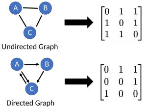
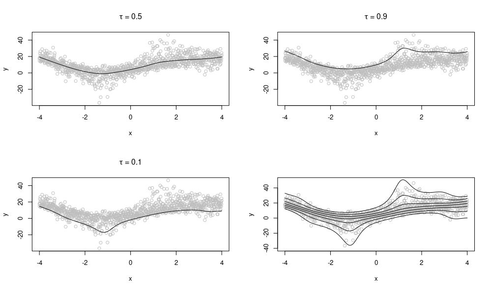
QGAMs are essentially the result of combining quantile regression (QR; performing regression on a specific quantile of the response) with a generalised additive model (GAM; fitting a model assuming additive smooth effects). Here we are in the regression setting, so let $F(y| \boldsymbol{x})$ be the conditional c.d.f. of a response, $y$ , given a $p$ -dimensional vector of covariates, $\boldsymbol{x}$ . In QR we model the $\tau$ th quantile, that is, $\mu_\tau(\boldsymbol{x}) = \inf \{y : F(y|\boldsymbol{x}) \geq \tau\}$ .

Examples of true quantiles of SHASH distribution.

This might be useful in cases where we do not need to model the full distribution of $y| \boldsymbol{x}$ and only need one particular quantile of interest (for example urban planners might only be interested in estimates of extreme rainfall e.g. $\tau = 0.95$ ). It also allows us to make no assumptions about the underlying true distribution, instead we can model the distribution empirically using multiple quantiles.

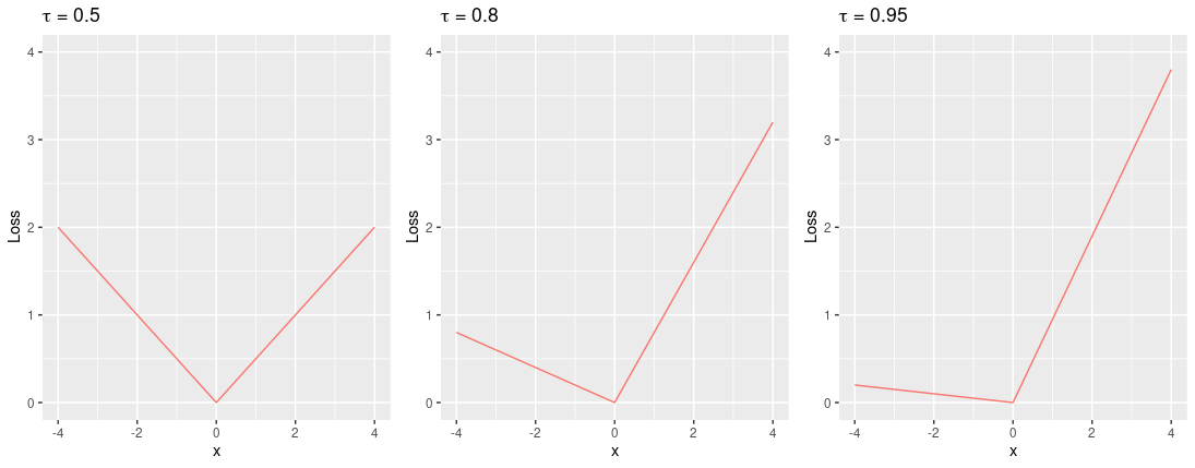
We can define the $\tau$ th quantile as the minimiser of expected loss

$L(\mu| \boldsymbol{x}) = \mathbb{E} \left\{\rho_\tau (y - \mu)| \boldsymbol{x} \right \} = \int \rho_\tau(y - \mu) d F(y|\boldsymbol{x}),$

w.r.t. $\mu = \mu_\tau(\boldsymbol{x})$ , where

$\rho_\tau (z) = (\tau - 1) z \boldsymbol{1}(z<0) + \tau z \boldsymbol{1}(z \geq 0),$

is known as the pinball loss (Koenker, 2005).

Pinball loss for quantiles 0.5, 0.8, 0.95.

We can approximate the above expression empirically given a sample of size $n$ , which gives the quantile estimator, $\hat{\mu}_\tau(\boldsymbol{x}) = \boldsymbol{x}^\mathsf{T} \hat{\boldsymbol{\beta}}$ where

$\hat{\boldsymbol{\beta}} = \underset{\boldsymbol{\beta}}{\arg \min} \frac{1}{n} \sum_{i=1}^n \rho_\tau \left\{y_i - \boldsymbol{x}_i^\mathsf{T} \boldsymbol{\beta}\right\},$

where $\boldsymbol{x}_i$ is the $i$ th vector of covariates, and $\boldsymbol{\beta}$ is vector of regression coefficients.

So far we have described QR, so to turn this into a QGAM we assume $\mu_\tau(\boldsymbol{x})$ has additive structure, that is, we can write the $\tau$ th conditional quantile as

$\mu_\tau(\boldsymbol{x}) = \sum_{j=1}^m f_j(\boldsymbol{x}),$

where the $m$ additive terms are defined in terms of basis functions (e.g. spline bases). A marginal smooth effect could be, for example

$f_j(\boldsymbol{x}) = \sum_{k=1}^{r_j} \beta_{jk} b_{jk}(x_j),$

where $\beta_{jk}$ are unknown coefficients, $b_{jk}(x_j)$ are known spline basis functions and $r_j$ is the basis dimension.

Denote $\boldsymbol{\mathrm{x}}_i$ the vector of basis functions evaluated at $\boldsymbol{x}_i$ , then the $n \times d$ design matrix $\boldsymbol{\mathrm{X}}$ is defined as having $i$ th row $\boldsymbol{\mathrm{x}}_i$ , for $i = 1, \dots, n$ , and $d = r_1+\dots +r_m$ is the total basis dimension over all $f_j$ . Now the quantile estimate is defined as $\mu_\tau(\boldsymbol{x}_i) = \boldsymbol{\mathrm{x}}_i^\mathsf{T} \boldsymbol{\beta}$ . When estimating the regression coefficients, we put a ridge penalty on $\boldsymbol{\beta}_{j}$ to control complexity of $f_j$ , thus we seek to minimise the penalised pinball loss

$V(\boldsymbol{\beta},\boldsymbol{\gamma},\sigma) = \sum_{i=1}^n \frac{1}{\sigma} \rho_\tau \left\{y_i - \mu(\boldsymbol{x}_i)\right\} + \frac{1}{2} \sum_{j=1}^m \gamma_j \boldsymbol{\beta}^\mathsf{T} \boldsymbol{\mathrm{S}}_j \boldsymbol{\beta},$

where $\boldsymbol{\gamma} = (\gamma_1,\dots,\gamma_m)$ is a vector of positive smoothing parameters, $1/\sigma>0$ is the learning rate and the $\boldsymbol{\mathrm{S}}_j$ ‘s are positive semi-definite matrices which penalise the wiggliness of the corresponding effect $f_j$ . Minimising $V$ with respect to $\boldsymbol{\beta}$ given fixed $\sigma$ and $\boldsymbol{\gamma}$ leads to the maximum a posteriori (MAP) estimator $\hat{\boldsymbol{\beta}}$ .

There are a number of methods to tune the smoothing parameters and learning rate. The framework from Fasiolo et al. (2021) consists in:

calibrating $\sigma$ by Integrated Kullback–Leibler minimisation
selecting $\boldsymbol{\gamma}|\sigma$ by Laplace Approximate Marginal Loss minimisation
estimating $\boldsymbol{\beta}|\boldsymbol{\gamma},\sigma$ by minimising penalised Extended Log-F loss (note that this loss is simply a smoothed version of the pinball loss introduced above)

For more detail on what each of these steps means I refer the reader to Fasiolo et al. (2021). Clearly this three-layered nested optimisation can take a long time to converge, especially in cases where we have large datasets which is often the case for energy demand forecasting. So my project approach is to adapt this framework in order to make it less computationally expensive.

Application to Swiss Extreme Rainfall

Here I will briefly discuss one potential application of QGAMs, where we analyse a dataset consisting of observations of the most extreme 12 hourly total rainfall each year for 65 Swiss weather stations between 1981-2015. This data set can be found in the R package gamair and for model fitting I used the package mgcViz.

A basic QGAM for the 50% quantile (i.e. $\tau = 0.5$ ) can be fitted using the following formula

$\mu_i = \beta + \psi(\mathrm{reg}_i) + f_1(\mathrm{nao}_i) + f_2(\mathrm{el}_i) + f_3(\mathrm{Y}_i) + f_4(\mathrm{E}_i,\mathrm{N}_i),$

where $\beta$ is the intercept term, $\psi(\mathrm{reg}_i)$ is a parametric factor for climate region, $f_1, \dots, f_4$ are smooth effects, $\mathrm{nao}_i$ is the Annual North Atlantic Oscillation index, $\mathrm{el}_i$ is the metres above sea level, $\mathrm{Y}_i$ is the year of observation, and $\mathrm{E}_i$ and $\mathrm{N}_i$ are the degrees east and north respectively.

After fitting in mgcViz, we can plot the smooth effects and see how these affect the extreme yearly rainfall in Switzerland.

Fitted smooth effects for North Atlantic Oscillation index, elevation, degrees east and north and year of observation.

From the plots observe the following; as we increase the NAO index we observe a somewhat oscillatory effect on extreme rainfall; when increasing elevation we see a steady increase in extreme rainfall before a sharp drop after an elevation of around 2500 metres; as years increase we see a relatively flat effect on extreme rainfall indicating the extreme rainfall patterns might not change much over time (hopefully the reader won’t regard this as evidence against climate change); and from the spatial plot we see that the south-east of Switzerland appears to be more prone to more heavy extreme rainfall.

We could also look into fitting a 3D spatio-temporal tensor product effect, using the following formula

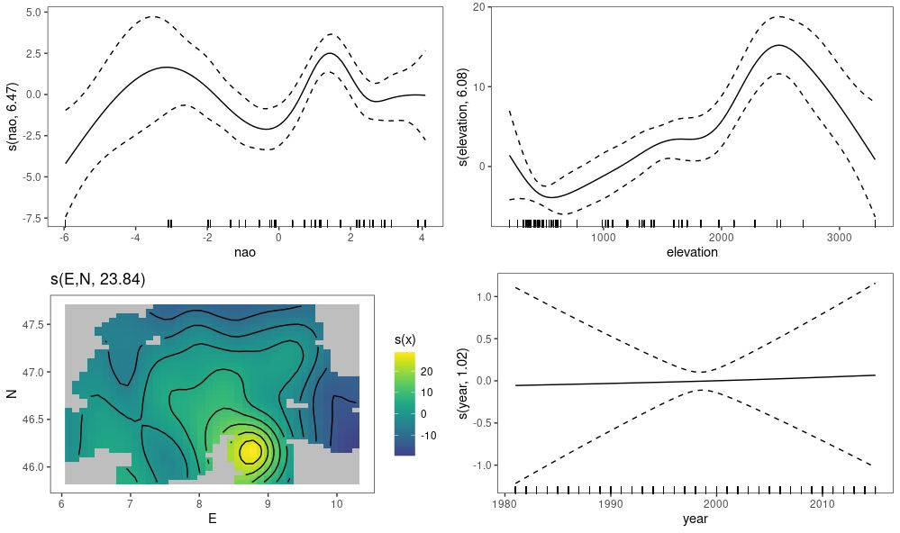
$\mu_i = \beta + \psi(\mathrm{reg}_i) + f_1(\mathrm{nao}_i) + f_2(\mathrm{el}_i) + t(\mathrm{E}_i,\mathrm{N}_i,\mathrm{Y}_i),$

where $t$ is the tensor product effect between $\mathrm{E}_i$ , $\mathrm{N}_i$ and $\mathrm{Y}_i$ . We can examine the spatial effect on extreme rainfall over time by plotting the smooths.

3D spatio-temporal tensor smooths for years 1985, 1995, 2005 and 2015.

There does not seem to be a significant interaction between the location and year, since we see little change between the plots, except for perhaps a slight decrease in the south-east.

Finally, we can make the most of the QGAM framework by fitting multiple quantiles at once. Here we fit the first formula for quantiles $\tau = 0.1, 0.2, \dots, 0.9$ , and we can examine the fitted smooths for each quantile on the spatial effect.

Spatial smooths for quantiles 0.1, 0.2, …, 0.9.

Interestingly the spatial effect is much stronger in higher quantiles than in the lower ones, where we see a relatively weak effect at the 0.1 quantile, and a very strong effect at the 0.9 quantile ranging between around -30 and +60.

The example discussed here is but one of many potential applications of QGAMs. As mentioned in the introduction, my research area is motivated by energy demand forecasting. My current/future research is focused on adapting the QGAM fitting framework to obtain faster fitting.

References

Fasiolo, M., S. N. Wood, M. Zaffran, R. Nedellec, and Y. Goude (2021). Fast calibrated additive quantile regression. Journal of the American Statistical Association 116 (535), 1402–1412.

Koenker, R. (2005). Quantile Regression. Cambridge University Press.

Student perspectives: ensemble modelling for probabilistic volcanic ash hazard forecasting

Posted on 23rd September 202222nd November 2022 by shannon.williams

A post by Shannon Williams, PhD student on the Compass programme.

My PhD focuses on the application of statistical methods to volcanic hazard forecasting. This research is jointly supervised by Professor Jeremy Philips (School of Earth Sciences) and Professor Anthony Lee. (more…)

Student Perspectives: An introduction to normalising flows

Posted on 13th July 202222nd November 2022 by Dan Ward

A post by Dan Ward, PhD student on the Compass programme.

Normalising flows are black-box approximators of continuous probability distributions, that can facilitate both efficient density evaluation and sampling. They function by learning a bijective transformation that maps between a complex target distribution and a simple distribution with matching dimension, such as a standard multivariate Gaussian distribution. (more…)

Student perspectives: Neural Point Processes for Statistical Seismology

Posted on 20th June 202210th August 2022 by sam.stockman

A post by Sam Stockman, PhD student on the Compass programme.

Introduction

Throughout my PhD I aim to bridge a gap between advances made in the machine learning community and the age-old problem of earthquake forecasting. In this cross-disciplinary work with Max Werner from the School of Earth Sciences and Dan Lawson from the School of Mathematics, I hope to create more powerful, efficient and robust models for forecasting, that can make earthquake prone areas safer for their inhabitants.

For years seismologists have sought to model the structure and dynamics of the earth in order to make predictions about earthquakes. They have mapped out the structure of fault lines and conducted experiments in the lab where they submit rock to great amounts of force in order to simulate plate tectonics on a small scale. Yet when trying to forecast earthquakes on a short time scale (that’s hours and days, not tens of years), these models based on the knowledge of the underlying physics are regularly outperformed by models that are statistically motivated. In statistical seismology we seek to make predictions through looking at distributions of the times, locations and magnitudes of earthquakes and use them to forecast the future.

(more…)